Tuning Spatial Profiles of Selection Pressure to Modulate the Evolution of Drug Resistance

Introduction

Understanding microbial antibiotic resistance is a daunting task, as bacteria grow in complex environments with a myriad of different environmental parameters that can affect their growth rate, such as pH, temperature, density, drug distribution, and nutrient distribution, just to name a few. In many laboratory experiments of bacteria, many of these factors are carefully controlled for to allow scientists to isolate the effects of the quantities of interest. However, can spatial variation in these often-neglected quantities impact the emergence of antibiotic resistance? In our PRL paper, we find that spatial variation in such factors can significantly impact the emergence of fixation. Importantly, variation in such factors can either speed or slow fixation depending on the region of parameter space, even while conserving the spatially-averaged value of such factors. In this post, I hope to provide a more thorough introduction to the model we developed than is possible given the space constraints of a manuscript. My goal is to provide the interested reader who may not be an expert in the field with enough background information to better understand the model introduced in the paper and the subsequent results.

Emergent Behavior

Before I introduce the model I developed, I want to briefly explain the philosphy motivating this model. Any model of physical phenomena necessarily discards some information. Every scientist creating a model has to balance the (potentially) competing goals of accurate replication and number of model parameters. For certain problems demanding realistic simulations, high-fidelity models including as many parameters as possibly relevant are the optimal solution. The model I developed is on the other side of the fidelity spectrum. The model I develop for microbial evolution is a toy model, exchanging realistic population characterization for a small number of parameters. These toy models can be surprisingly useful in complicated systems due to emergent behavior. Emergent behavior is a very general term used to describe situations in which a large number of microscopic units can lead to unexpected behavior on the macroscopic scale due to simple interactions.

As one example of emergent behavior, a common model of magnetism treats individual atoms as simple magnetic dipoles, with a binary spin pointing either up or down. These magnetic spins obey simple interaction with neighboring spins. Despite the simple characterization of atoms and their interactions, the macroscopic phenomenon that we call “magnetism” emerges from a very large number of these simple constituent units. This macroscopic behavior is difficult to predict if we only think about how two neighboring spins interact. And crucially, we end up with a very good model of magnetism despite the very large amount of information we are neglecting about individual atoms.

Emergent behavior is commonly observed in many contexts, including biophysics. For antibiotic resistance, scientists understand a large number of molecular mechanisms that confer resistance to individual bacteria cells. This project looks at the resulting dynamics of a large population of bacteria that are not immediately obvious from only understanding single drug-cell interactions. We do not intend to accurately model all of the complexities of bacteria or antibiotics but instead create a toy model using a simple set of rules that still exhibits rich dynamics. And because the system is very simple with relatively few parameters, we can much easier interpret the model and gain an intuition behind the observed behavior.

Toy Model of Bacteria

Our first big assumption in our model is that there exist two types of cells—those sensitive to some drug present and those resistant to it. The drug is a bacteristatic agent, meaning that it inhibits the growth of sensitive cells but does not kill them. This means that the resistant cells will grow faster than the sensitive cells, but both die at the same rate. In addition to cell replication, we add the possibility of mutation, in which a sensitive cell can become resistant. We treat population growth as a Moran process, so that the total population of cells is constant. At every timestep, one cell is chosen to replicate and one cell is chosen to die.

To introduce spatial structure into our model, we assume that the evolution is occuring in multiple well-mixed populations. Within each of these microhabitats, all cells of the same type are equivalent and the effectiveness of the drug is constant. The spatial structure comes from multiple microhabitats connected to allow migration of cells. Thus, the sytem we are interested looks something like the cartoon shown below. Note that we can have differing drug concentrations in the three different vials, so that not all of the microhabitats are equivalent.

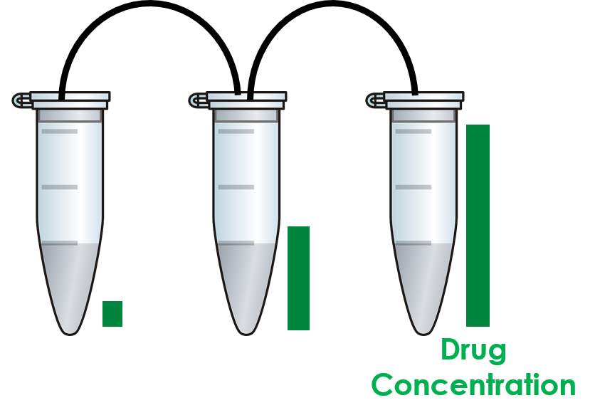Cartoon illustrating three connected microhabitats.

With these rules in place, we can write down different states in our system and the transitions between them. Since we assume that the population size is fixed and that the drug concentrations are constant, our state is completely defined by the number of mutant cells in each of the three microhabitats. Mathematically, we denote the microhabitats with spatial coordinates $x_i$ and the number of mutants in each microhabitat as $n^*(x_i)$. The full state is thus given by the tuple $(n^*(x_0), n^*(x_1), n^*(x_2))$.

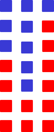Illustrative example of the state (4, 2, 6) if blue squares represent sensitive cells and red represent resistant cells.

To introduce dynamics into our system, we need to understand how states change in time. Because of our Moran process assumption, the number of mutants in each microhabitat can change by at most one in a single timestep. So with three microhabitats, there are six new states that can be reached in a given timestep.

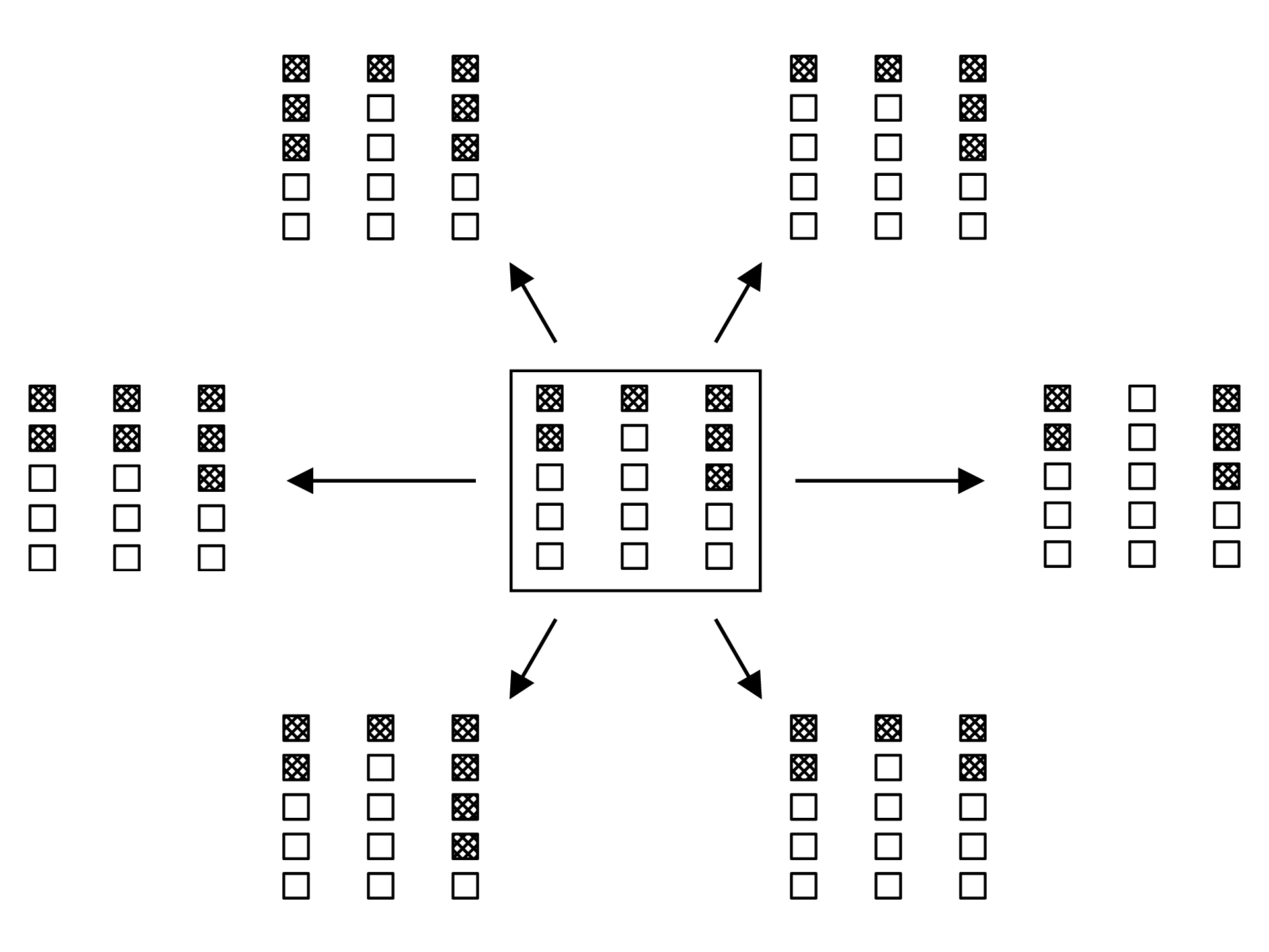For a general state of the system, shown in the center, six new states can be reached in a single timestep.

Before we can describe the transitions between states in our system, we need to introduce a few more parameters into our system. Let’s first fully define the two types of cells in our system. We assume each microhabitat $x_i$ has $N$ total cells, of which $n_0(x_i)$ are sensitive cells and $n^*(x_i)$ are resistant. We also need to define the growth rates of both sensitive and resistant cells. We assume that the mutants are completely uninhibited by the presence of drug, so that they have the maximum fitness of $r^*(x_i) = 1$. The sensitive cells, however, grow more slowly in the presence of drug, so that they have a fitness given by $0 < r_0(x_i) \leq 1$. Because the spatial distribution of drug can vary between microhabitats, the fitness of the sensitive cells can also vary between microhabitats. This motivates the definition of selection pressure, which physically quantifies how advantageous mutant cells are over sensitive cells. We define selection pressure as $$\displaylines{\begin{align} s(x_i) &= r^*(x_i) - r_0(x_i) \\ &= 1 - r_0(x_i) \end{align}}$$ This definition helps explain the first part of the title of this paper. We have now introduced the idea of a spatial selection pressure landscape. To understand the evolution of drug resistance with a given selection pressure landscape, we need to introduce two more important parameters. First, I earlier mentioned that we allow sensitive cells to mutate into the drug-resistant cells. This is a stochastic process occurring at rate $\mu$. I also have mentioned that cells can migrate to neighboring microhabitats. This is also stochastic and occurs at rate $\beta$.

We now have introduced everything that we need to define the transitions between states in our system. We will start by writing down the complete transition rate that increases the number of mutants in the center microhabitat, which we denote as $T^+[x_1](n^*(x_0), n^*(x_1), n^*(x_2))$. Before we write down the full transition rate, let’s think about what could happen that would increase the number of mutant cells in our center microhabitat. Because of our constant population size assumption, we require both a sensitive cell to die and the addition of a mutant. One possibility is that we have an existing mutant cell replicate and that the daughter cell does not migrate to a neighboring microhabitat. Upon weighting mutant replication by both the number of mutant cells and the mutant fitness, this process introduces a term $$n_0(x_1) \frac{n^*(x_1)}{N} \frac{r^*(x_1)}{\bar{r}(x_1)} (1 - 2 \beta), $$ where we make use of the mean fitness $\bar{r}(x_1)$ given by $$ \bar{r}(x_1) = \frac{n^*(x_1) r^*(x_1) + n_0(x_1) r_0(x_1)}{N}. $$ Another possible mechanism is that an existing sensitive cell mutates. The replication is weighted by the sensitive cell fitness, producing a contribution $$n_0(x_1) \frac{n_0(x_1)}{N} \frac{r_0(x_1)}{\bar{r}(x_1)} \mu. $$ Finally, we also must account for the possibility of a mutant cell in a neighboring microhabitat replicating and the daughter cell migrating into the center microhabitat. The contribution due to the left-neighboring microhabitat is given by $$n_0(x_1) \frac{n^*(x_0)}{N} \frac{r^*(x_0)}{\bar{r}(x_0)} \beta, $$ and we have an analagous term due to migrants from the right-neighboring microhabitat. Upon combining all of these contributions, we have a transition rate given by $$\begin{multline} T^+[x_1](n^*(x_0), n^*(x_1), n^*(x_2)) = n_0(x_1) \Bigg[ \frac{n^*(x_1)}{N} \frac{r^*(x_1)}{\bar{r}(x_1)} (1 - 2 \beta) + \frac{n_0(x_1)}{N} \frac{r_0(x_1)}{\bar{r}(x_1)} \mu + \\ \frac{n^*(x_0)}{N} \frac{r^*(x_0)}{\bar{r}(x_0)} \beta + \frac{n^*(x_2)}{N} \frac{r^*(x_2)}{\bar{r}(x_2)} \beta \Bigg]\end{multline}. $$ The terms increasing the number of mutants in the left and right microhabitats take a very similar form, although they have one less term since they only have one neighboring microhabitat.

We can perform the same accounting for determining the transition rate decreasing the number of mutants in the center microhabitat. Let’s enumerate over the processes that reduce the number of mutants and build up this transition rate term by term. We can first decrease the number of mutants by choosing a mutant cell to die and having a sensitive cell replicate without mutation or migration. This yields the term $$ n^*(x_1) \frac{n_0(x_1)}{N} \frac{r_0(x_1)}{\bar{r}(x_1)} (1 - \mu - 2 \beta). $$ We can also have a sensitive cell migrate into the center microhabitat. For the left-neighboring microhabitat, this produces the term $$ n^*(x_1) \frac{n_0(x_0)}{N} \frac{r_0(x_0)}{\bar{r}(x_0)} \beta, $$ and we have an analagous term for sensitive cells from the right-neighboring microhabitat. Collectively, these terms produce the transition rate $$\begin{multline}T^-[x_1](n^*(x_0), n^*(x_1), n^*(x_2)) = n^*(x_1) \Bigg[ \frac{n_0(x_1)}{N} \frac{r_0(x_1)}{\bar{r}(x_1)} (1 - \mu - 2 \beta) + \frac{n_0(x_0)}{N} \frac{r_0(x_0)}{\bar{r}(x_0)} \beta \\ + \frac{n_2(x_2)}{N} \frac{r_2(x_2)}{\bar{r}(x_2)} \beta \Bigg].\end{multline} $$ We will again have very similar expressions for the transition rates for the other microhabitats. With these transition rates constructed, our toy model of evolution is completely specified.

Studying Fixation

At this point, we have developed a simple model of stochastic evolution in which the state of the system can transition to different states at known rates. And due to the assumption of a Moran process, relatively few new states can be reached in a single timestep. To understand the dynamics resulting from these transition rates, we borrow the idea of a master equation from statistical physics. Writing down our system as a master equation provides us with a set of differential equations that can be solved to tell us about how the system evolves in time.

We first need to write down the transition rate matrix for our system, also called the master equation operator. This is easily formed by organizing the transition rates that we have formed above. Recall that the state of our system is given by the number of mutants in each of the three microhabitats, so that an arbitrary state $m$ is given by $(n^*(x_0), n^*(x_1), n^*(x_2))$. If we briefly depart from our earlier notation and use $W^{m' \rightarrow m}$ to denote the transition rate from initial state $m'$ to final state $m$, the transition rate matrix $\Omega_{m m'}$ for our system is given by $$\Omega_{m m’} = \begin{cases} W^{m’ \rightarrow m} &\qquad m \neq m’ \\ -\sum_{\ell \neq m} W^{m \rightarrow \ell} &\qquad m = m’. \end{cases} $$ It is worth pointing out here that our transition matrix is sparse, since the majority of possible states are not reachable from an arbitrary initial state in a single timestep. This has important consequences for our ability to solve for the qualities of interest in our system, as we will see. To start, we will use the transition matrix we have developed to write down an expression containing $P_m(t)$, the probability of the system being in state $m$ at time $t$. This obeys the master equation $$\frac{d P_m}{d t} = \sum_{m’} \Omega_{m m’} P_{m’}. $$ This gives us a system of coupled differential equations that when solved tells us the probability of our system being in state $m$ at any arbitrary time $t$. However, the resulting differential equations produced by a master equation are often not analytically solvable due to nonlinearities in the transition rates, and our problem is no exception. In many problems modeled using a master equation, an acceptable compromise is to calculate the stationary probability distribution, as the transients of the system are often not of primary interest. For our system, however, we already know the stationary probability distribution. Because we allow mutations from the sensitive cells to resistant cells but not the reverse process, the state $(N, N, N)$, in which all microhabitats are composed entirly of mutants, is an “absorbing state,” meaning that the state of the system cannot change once this state is reached. If the system evolves for long enough, we are guaranteed to reach this all-mutant state. Physically, this state is interesting to us because it is the state corresponding to complete mutant fixation.

So if we cannot solve the master equation for our system to learn something useful, what can we hope to accomplish? One idea is to measure how long the system takes to reach this inevitable fixation state. We can hope to characterize the amount of time required to reach our absorbing fixation state from an initial state composed of entirely sensitive cells. We call this the fixation time, denoted by $\tau_f$. Our goal is to first be able to calculate $\tau_f$ for an arbitrary selection landscape and then secondly to understand how the parameters of the system affect this fixation time.

To calculate our fixation time, we return to our master equation operator $\Omega$. It is related to $T(m_f \vert m')$, the mean time required to reach a final state $m_f$ from an initial state $m'$. This quantity is called the mean first passage time, and it is related to our master equation operator by the equation $$-1 = \sum_{m’ \neq m_f} T(m_f \vert m’) \Omega_{m’ m_i}.$$ This provides us with a coupled set of equations that we can solve to calculate $\tau_f = T((N, N, N) \vert (0, 0, 0)) $. To illustrate the calculation, let’s write down the equation for $m_f = (N, N, N)$ and $m_i = (0, 0, 0)$. In this case, we sum over all possible other states $m'$, but the only states that will not be multiplied by zero from our master equation operator are those that can be reached in a single timestep from the initial state $m_i = (0, 0, 0)$. So this leaves us with the equation $$\displaylines{\begin{multline} -1 = T((N, N, N) \vert (0, 0, 0)) \Omega_{(0, 0, 0), (0, 0, 0)} + T((N, N, N) \vert (1, 0, 0)) \Omega_{(1, 0, 0), (0, 0, 0)} + \\ T((N, N, N) \vert (0, 1, 0)) \Omega_{(0, 1, 0), (0, 0, 0)} + T((N, N, N) \vert (0, 0, 1)) \Omega_{(0, 0, 1), (0, 0, 0)}. \end{multline}}$$ Using our transition rates, we can write this as $$\displaylines{\begin{multline} -1 = -\tau_f \Big(T^+[x_0](0, 0, 0) + T^+[x_1](0, 0, 0) + T^+[x_2](0, 0, 0)\Big) + \\ T((N, N, N) \vert (1, 0, 0)) T^+[x_0](0, 0, 0) + T((N, N, N) \vert (0, 1, 0)) T^+[x_1](0, 0, 0) + \\ T((N, N, N) \vert (0, 0, 1)) T^+[x_2](0, 0, 1).\end{multline}} $$ This equation relates the transition rates to the mean first passage times that we want to solve for. However, note that we currently have four unknown quantities for a single equation, so we cannot solve for $\tau_f$ just yet. Instead, we need to introduce more equations by choosing a different value for our initial state $m_i$. But these additional equations come with additional unknown quantities in the form of unknown mean first passage times. In total, how many mean first passage times are there to solve for? Each microhabitat can take any number of mutants between 0 and $N$, so there are a total of $(N + 1)^3$ unique states for our system. For each of these states, we can form a mean first passage time to calculate the average time required to first reach the state $m_f = (N, N, N)$. All of these states will therefore have a corresponding unknown mean first passage time, with the exception of the state of fixation, since we have $T((N, N, N) \vert (N, N, N)) = 0$ by definition. Our initial state $m_i$ is allowed to take any of the possible states with the exception of $m_f$, so we will have exactly the same number of equations. This works great, since we have $(N + 1)^3 - 1$ equations for the same number of unknowns, even if the accounting gets messy.

Now that we know that the system of equations can in theory be solved, how do we go about doing this? The first concern lies with our master equation operator $\Omega$. Since each state is represented by a 3-tuple, the most natural formulation for our master equation operator would be a sixth-order tensor, which would be difficult to work with in standard linear algebra libraries. So our first task is to create a mapping between the natural 3-tuple representation of our state to a unique integer. This mapping is not inherently interesting and can be completely arbitrary, so I will skip describing it in favor of simply showing our master equation operator $\Omega$ expressed as a sparse matrix for a very small system with $N = 2$.

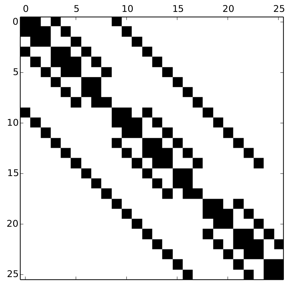Our master equation operator $\Omega$ written as a sparse matrix, with black entries denoting non-zero elements.

The fact that our master equation operator is sparse contributes greatly to the computational feasability of solving for $\tau_f$. For many of the results in our published paper, we used a system size of $N = 25$. This means that a dense master equation operator would contain more than 300 million entries. Populating this operator would be time consuming, as would any meaningful calculation using it. Instead, the Moran process assumption means that a general state can reach a total of six new states. Written as a sparse matrix, the master equation operator for our system contains fewer than 36,000 elements. We can very easily perform linear algebra operations on a matrix of this size.

Let’s now think about the linear algebra operations we need to perform to solve for our mean first passage times. As we already saw, although we are only interested in the fixation time from the initial sensitive state, $\tau_f$, we necessarily have to calculate all of the other mean fixation times. We can take advantage of sparse linear algebra routines by vectorizing our sytem of equations. We can form the mean fixation time vector $$ \mathbf{T} = \begin{pmatrix} T((N, N, N) \vert (0, 0, 0)) \\ \vdots \\ T((N, N, N) \vert (N, N, N - 1)) \end{pmatrix}. $$ We already have the master equation operator represented as a matrix, so we last need to introduce a ones vector $\mathbf{1}$. Our system can then be written as $$- \mathbf{1} = \Omega^T \mathbf{T}. $$ This is now in a form that can be solved with standard sparse linear algebra routines. Let’s look at the resulting vector of mean fixation times. We choose to organize the states according to their mutant fraction. Note that because we can have several states with the same mutant fraction, we can have several mean fixation times for the same mutant fraction. This is illustrated in the accompanying cartoon. The fixation times are plotted as a grey point for all possible initial states, with the mutant fraction on the x-axis and the normalized mean fixation times on the y-axis. The red line shows the average mean fixation time for a given mutant fraction, and this decreases monotonically as we would expect.

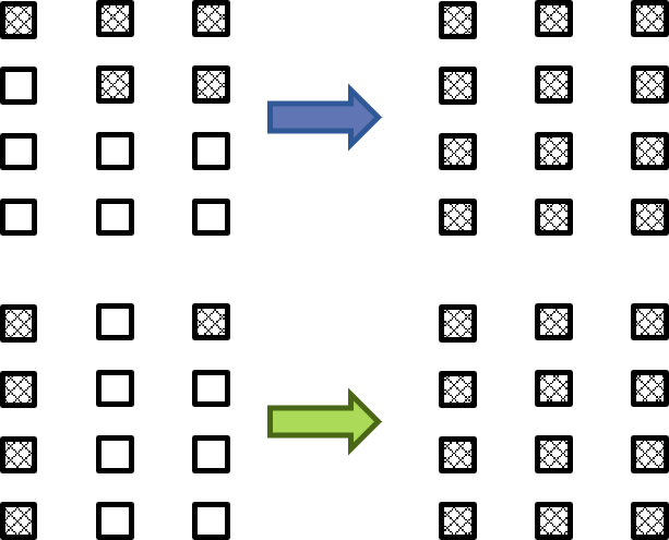We can form multiple states with the same mutant fraction.

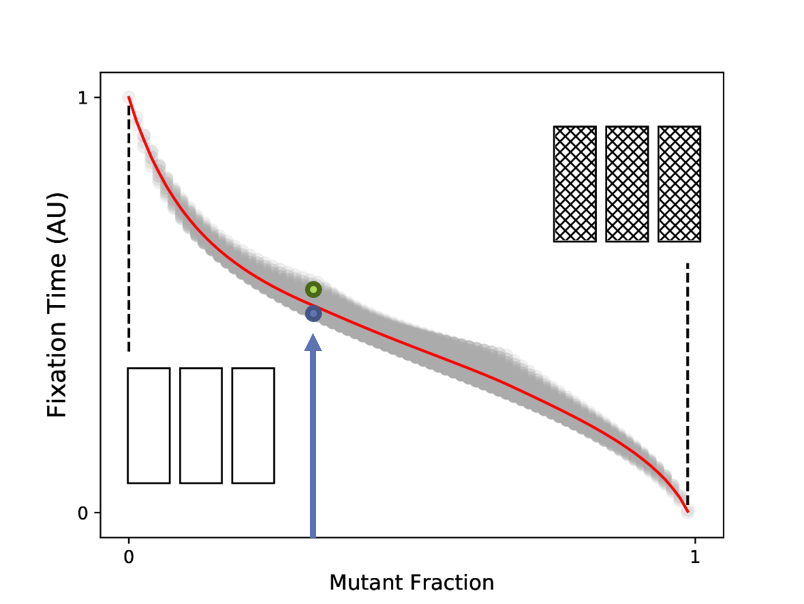Plotting the resulting vector $\mathbf{T}$ after organizing states according to their mutant fraction.

In general, we are mostly interested in the time required for an initially sensitive population to be entirely composed of mutants, $\tau_f$. This is the single datapoint corresponding to zero initial mutant fraction in the above figure. Now that we have a procedure for calculating this mean fixation time, we can vary the parameters of the system to understand how they impact the time to resistance.

Classes of Selection Landscapes

For a given population size $N$, mutation rate $\mu$, and migration rate $\beta$, the only unspecified aspect of the system is the selection pressure landscape. Physically, we can think of a spatial distribution of drug generating this selection landscape. We want to be careful about how we compare fixation times across different selection landscapes. It is intuitively obvious that we can affect the time to resistance by adding more total drug to one system. To isolate the effect of spatial distribution, we look at different classes of selection pressure landscapes that conserve the mean selection pressure $\langle s \rangle$.

We choose to model the selection pressure landscape as symmetric, with the left and right microhabitats having the same selection pressure values for any landscape. This is not a necessary assumption, but it reduces the number of free parameters in our system. And as we will see, our results are not predicated upon this assumption. With this constraint, we parameterize our selection landscapes by $$\delta s \equiv s(x_1) - s(x_0),$$ which physically tells us the selection pressure in the center microhabitat relative to either of the extrema microhabitats. If we have $\delta s > 0$, we have a spatial peak in our selection pressure landscape. And if we have $\delta s < 0$, we have a spatial valley in our selection landscape. The landscape with $\delta s = 0$ is the homogeneous selection landscape, in which all microhabitats have the same selection pressure. We can now fully specify a selection landscape with $\langle s \rangle$ and $\delta s$.

We will first fix our mutation and migration rates to $\mu = 10^{-3}$ and $\beta = 10^{-3}$ and varying $\delta s$ to explore different selection landscapes with $N = 25$. For each of these landscapes, we perform the calculation detailed above, and we plot the value of $\tau_f$ resulting from each landscape in the figure below. Interestingly, the resulting fixation times can be faster or slower than what is obtained with the homogeneous landscape depending on the value of $\delta s$. And this is true despite conserving $\langle s \rangle$ across the landscapes. Physically, this can be thought of as having a fixed quantity of drug but changing the time to resistance simply by changing how it is distributed among the three microhabitats.

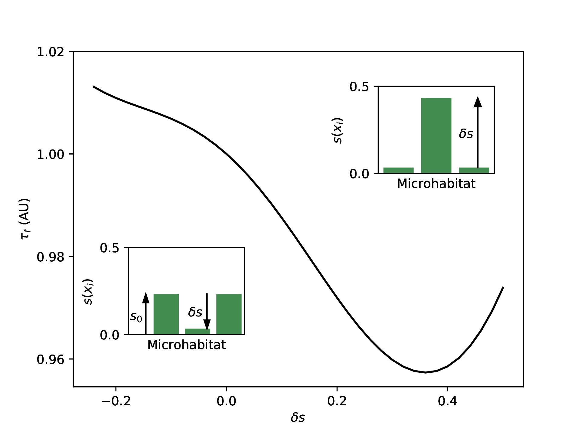Calculating the mean fixation time $\tau_f$ across different landscapes parameterized by $\delta s$ all conserving $\langle s \rangle $.

Behavior Across System Parameters

The above figure illustrates several interesting features, but by itself it is little more than a single case study. If we want to understand the effect of selection pressure landscapes on the emergence of resistance, we need to look over a broad range of values for our system parameters and characterize the types of behavior observed. Broadly, we can categorize the different spatial fixation time profiles into three distinct categories:

• A non-zero value for $\delta s$ always leads to a faster fixation time than in the homogeneous landscape with $\delta s = 0$. In these systems, spatial heterogeneity speeds the time to fixation.
• A non-zero value for $\delta s$ always leads to a slower fixation time than in the homogeneous landscape. In these systems, spatial heterogeneity slows the time to fixation.
• A non-zero value of $\delta s$ can lead to either faster or slow fixation compared to the homogeneous system depending on the value. This is what we observed in our figure above.

Our procedure to categorize the effect of spatial heterogeneity is now straightforward. For a given value of $\mu$ and $\beta$, we calculate the fixation times for all physical selection landscapes for a given value of $\langle s \rangle$. We require that all landscapes satisfy $0 < r_0(x_i) \leq 1$, which constrains the physical values of $\delta s$ to a finite range. Biologically, this assumption is equivalent to assuming that the sensitive cells are well-adapted to their initial drug-free environment, so they necessarily grow worse in the presence of drug. Once we have the profile of spatial fixation times across valid values of $\delta s$, we assign the particular choice of parameters $\mu$ and $\beta$ to one of our three mutually-exclusive categories. By systematically varying both $\mu$ and $\beta$ across several orders of magnitude, we can hope to learn something about the effect of these parameters on the fixation times in our system. After performing this procedure, we produce the figure below.

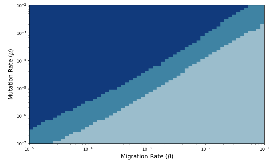Categorizing the effect of spatial heterogeneity across $\mu$–$\beta$ space. Broadly, we see that there are regions of parameter space where heterogeneity always speeds fixation, always slows fixation, and can either speed or slow fixation depending on the value of $\delta s$.

We see that the different regions are organized according to the relative magnitude of our mutation rate $\mu$ and migration rate $\beta$. Generally, when the mutation rate is small relative to the migration rate, the system is in the dark blue region of parameter space where heterogeneity speeds fixation. And when the migration rate is small relative to the mutation rate, the system lies in the light blue region of parameter space where heterogeneity slows fixation. Separating these two regions lies the intermediate region, where fixation can be both sped up and slowed down by heterogeneity in our selection landscape. The behavior of the system in these three regions of parameter space can be understood rigorously with the aid of an analytical model that we developed that approximates the dynamics of the system. In the interest of space, I will leave out the details of this approximation here but will instead describe the intuition behind the existence of these different regions of parameter space.

Let’s first look at the limiting case where we have $\beta \ll \mu$. In this limit, there is negligible migration between neighboring microhabitats, so we essentially have three independent systems concurrently evolving. The entire system does not reach fixation, however, until the slowest of these three independent system reaches fixation. Upon introducing spatial heterogeneity into the system, there will be at least one microhabitat with a smaller selection pressure and at least one with a large selection pressure than in the spatially-homogeneous system. Any microhabitat with a larger value of selection pressure will preferentially favor mutant cells more strongly than a microhabitat with a smaller value of selection pressure. As the system evolves according to biased genetic drift, the mutants will more quickly outcompete the sensitive cells in the larger selection pressure microhabitat. But in the smaller selection pressure microhabitat, the opposite effect is occuring, and fixation in this microhabitat will be slower compared to the spatially homogeneous system. Because we conserve our mean selection pressure, we necessarily generate a microhabitat with a smaller selection pressure by introducing spatial heterogeneity, and this rate-limits fixation in the entire system.

Let’s next look at the limiting case where we have $\mu \ll \beta$. In this limit, a very significant contribution to the fixation time of the system comes from waiting for the first mutation to occur. After this mutation arises, the mutant subpopulation will relatively quickly spread to the other microhabitats. However, the system is still evolving according to biased genetic drift, so it is possible for the mutant subpopulation to go extinct before it takes over the system. An extinction would require another long period of waiting for the next mutation event. The probability of a small mutant subpopulation is inversely related to the selection pressure in its respective microhabitat—with a small selection pressure value, the mutant cells are only slightly advantageous to the sensitive cells, and there is a good chance a small mutant subpopuation will die out due to genetic drift. The opposite is also true—with a large selection pressure value, the mutant cells are less likely to go extinct due to genetic drift. By adding spatial heterogeneity, we create both microhabitats with a larger and smaller selection pressure than in the homogeneous selection landscape. The existence of at least one microhabitat with a larger selection pressure reduces the likilihood of a small mutant subpopulation from going extinct, and this leads to a faster overall mean fixation time compared to the homogeneous landscape.

Concluding Thoughts

Already, we can begin to understand the importance of the selection pressure landscape on the emergence of resistance in this simple system. Even when the spatially-averaged selection pressure is fixed, its distribution can have large effects on the emergence of resistance. And if we want to know the size and direction of this effect, we need to know where our system lies in parameter space, since spatial heterogeneity can both speed or slow fixation, depending on the relative magnitude of the mutation rate and migration rate.

Initially, one might have thought that this artifical system we created was too simple to exhibit any of these interesting properties. This system has surprisingly rich dynamics that are not immediately intuitive, despite the very simple rules governing the cells. The simple model that I developed is a far cry from capturing the many complexities of anything resembling a realistic environment. However, we can learn from this simple model of the importance of spatial heterogeneity and begin to form an understanding of its impact on more realistic systems.

There is much more that I have learned about this model and its associated results than I have covered here. Some of these details are published our original PRL, and some await a future manuscript. Because this article is already very long, I’m going to end my discussion at this point. My goal is that this article equips the interested reader to understand the full paper and supporting material, which cover several exciting ideas that I will only briefly mention here. The first of two main ideas not covered is an analytical approximation to the fixation times in our system. We construct a statistical model that allows us to approximate fixation times using a much simpler calculation treating individual microhabitats as coupled random variables. This approximation also helps us to establish a rigorous intuition for the system. The second main idea deals with tuning the selection pressure landscape when we start with some non-zero number of mutants. Physically, this can loosely be thought of as trying to treat an existing infection by again changing the spatial drug distribution. We find that the time to resistance can again be significantly impacted by the distribution of selection and that the different treatment regimes can be intuitively understood despite the initially unanticipated results.