Lost Cities Part 2: Learning from Deep Q-Networks

In the previous article, we developed a reinforcement learning using deep Q-networks that was able to learn how to play Lost Cities. It achieved a mean score of 45 points per game, significantly outperforming a random agent. Can we probe this well-trained agent to understand its decision-making heuristics? Perhaps we could learn from this agent to improve our own ability at the game. Ultimately, we would like to play against it ourselves. Can it outperform a human opponent?

Trained Network Heuristics

Let’s first try to understand how the trained neural network plays the game. Rather than look at individual game states as case studies, let’s try to first understand its broad strategy choices. These macro-strategy choices are very easy to understand and reveal important information that is hard to gain from looking at how the network responds to any given state. To get data on the performance of the network, I evaluated the trained 5x512 network architecture to control the two opposing players for 5000 games. By recording the final played cards for both players, I had lots of data about how the trained agent approaches the game. First, let’s start with looking at the obtained joint scores of the two players. We see the trained scores in the below figure match what we were previously obtaining while training, which is a good sanity check. The mean score of 89.1 is very close to what we obtained from the network while training.

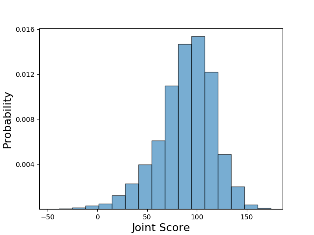The distribution of joint scores obtained from the trained agent, with the mean around 89 points.

Now let’s start to understand how the agents are achieving these scores. A very basic question is how many sets the agent starts. In the full rules of Lost Cities, each player is allowed to start any number of sets. However, the neural network is only allowed a single set per suit. This limitation was largely made for the sake of convenience, and it seems very reasonable given my own experience that starting two sets of the same suit are very rarely profitable. This is a very intuitive result, since each new set incurs a penalty of 20 points. Interestingly, in the figure below we see that the network almost plays all four possible sets. It only plays 3 sets in 0.3% of the games it played. This is the first odd result that differs from my experience of how a human plays the game. Because of the large cost incurred with each new stack, it can often be profitable for a player to devote his or her limited turns into fewer suits. This is especially true given the additional reward of 20 points given to sets of length 8 or greater.

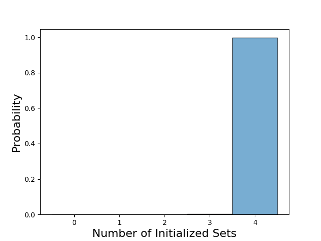The trained network almost exclusively intializes all four sets.

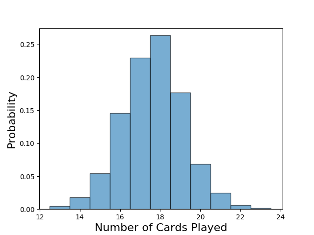
Because this strategy is unorthodox, the first thing we need to do is to ensure that the network achieving reasonable rewards is not using a strategy that would not work against other opponents. A game of Lost Cities is terminated when the final card is drawn. This means that the number of cards that the agent can play can vary. One strategy that is useful at times is to draw from the discarded cards rather than from the deck to extend the game. However, in the most pathologic case, the network could simply discard a card and then draw it again, so that the game never ends. In practice, we do not observe that this is an issue. However, it is still possible that the network abuses the discard pile to achieve unrealistic scores. With four sets of cards, generally getting to play more cards should lead to higher scores. Let’s first think about the bounds on the number of cards played. It is possible to play zero cards and achieve a score of zero points—the agent could always discard, and the opposing player could simply play as normal. For the upper bound, we can imagine being the opponent in this scenario. In this case, all of the cards except the 8 in our hand and in the hand of our opponent could be played, giving us an upper bound of 36 played cards. If we look at the distribution of played cards, we see that we are outside either of these two pathologic cases. The most common number of played cards is 18, which is what happens with both players play the same number of cards. This result is not particularly interesting on its own, but it suggests that the network is achieving impressive rewards using a strategy that is not completely unreasonable, even if it is unorthodox.

The trained network almost exclusively intializes all four sets.

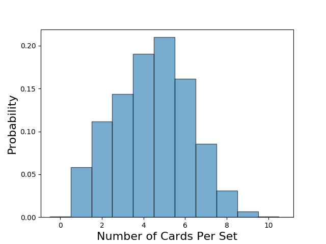
With the validity of the network’s strategy checked, let’s explore this curious strategy choice in more detail. First, we can look at the distribution of the number of cards in each set. We see that the network most often has five cards in a given set. It occasionally has a single card. This may seem initially troublesome, since the maximum possible reward from this set is -10 points. However, there are situations in which this is can occur under reasonable play. For example, a player may start a set but quickly cut his or her losses after failing to draw additional cards or seeing that the opposing player already has many cards in that suit. We also observe that the network rarely plays sets long enough to qualify for the +20 point bonus. Achieving a set with eight cards is challenging, but I suspect that the distribution resulting from my strategy would have significantly more than 3% of sets qualifying for the bonus. This is another significant strategy shift in the network, which does not seem to prioritize these longer sets. Of course, it is also entirely possible that the network just encounters such long sets too rarely in its training data to pursue them.

The trained network almost exclusively intializes all four sets.

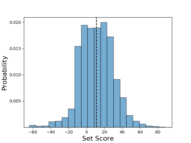
While we looked at the distribution of number of sets played and the number of cards per set, we are still missing some crucial information. Principally, we are missing the reward that the network gains from each set. We can calculate the score coming from all of the sets obtained over the 2000 games, and the distribution is shown below. Here, we start to see some very interesting information. Each set has a relatively wide distribution of scores, with the mean around 11 points. The distribution is fairly symmetric, although it has a longer tail for larger scores. Interestingly, the width of the distribution means that a significant number of sets fail to lead to positive scores. This is not surprising given the distribution of set length or the distribution of number of sets played.

The trained network almost exclusively intializes all four sets.

Piecing together these different plots, we start to get a sense of how the network approaches the game. The network almost exclusively plays four sets throughout the game. Each set is relatively short, which permits infrequent negative score contributions and also excludes reliance on the +20 point bonus received for sets of 8 cards. We see this clearly by looking at the CDF of the set scores below. However, under this strategy, each set provides +11 points in expectation. This number agrees closely with our result that the mean joint score is around 89 points.

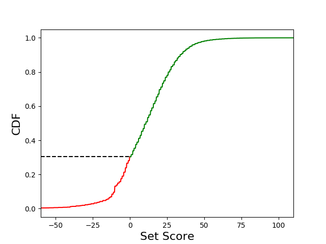The CDF of the set score distribution shows that roughly 70% of sets result in a positive score.

One way we can think about these results is to borrow from the idea of (coupled) biased random walks. If we were to treat the sets as uncoupled, which is certainly a poor assumption given the limited number of turns in a game, what is the probability that the score achieved is positive? We can answer this by Monte Carlo sampling our set score distribution. We find that the result of 4 individual sets is negative in only 12% of games. We can also look at what we obtain empirically, which does not require the assumption of independence between sets. We find that in practice, negative scores were obtained in 28% of games. This discrepancy is not surprising, since the scores between sets are strongly correlated. Although the scores obtained from the sets do not follow an uncoupled biased walk, it is still a useful analogy for intuition. Because the network was able to generate a set score distribution with a positive expected value, it samples it the maximum number of times to try to end up with a positive score.

This gets at an interesting question that is tied to our reward structure. It is possible that the optimization performed by the network resulted in a risk-averse strategy to avoid negative rewards. In our training, we used the score of the game as the reward function. Because negative rewards punish the agent, it is possible that the strategy found by the network represents an attempt to minimize the probability of negative rewards while still constrained to maximize score. If this were the case, the scores obtained would not truly be optimal if the network were too careful to avoid negative scores. This would explain, for example, why the network rarely achieved the +20 bonus score for long sets—establishing long sets typically relies on several multipliers, which greatly amplify the range of outcomes. Instead of attempt these lucrative strategies that have a possibility of resulting in large penalties from the reward function, the network takes a risk-averse strategy to reduce the number of negative rewards achieved. If we look at the distribution of multipliers played per set, we see below that more than 65% of the sets use zero or one multipliers. Does this distribution represent the optimal solution for a neural network to achieve the highest possible score, or is it merely the byproduct of the network trying to avoid negative rewards?

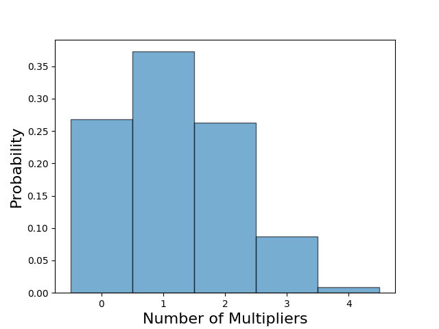The distribution of the number of multipliers played reveal that the network favors fewer multipliers.

To answer this and related questions, I retrained the network from scrach using the same architecture but providing an alternative reward function. We want to try a reward function that is less prone to producing a risk-averse network so that we can be certain that the score is being optimized properly. I modified the original reward function by adding 20 points upon the completion of the game. This number was chosen by looking at the distribution of set scores, which showed that the previous network very rarely received a score below -20. In a sense, we will now be tolerating more negative scores. If the trained network has significantly higher scores, we know that the above results are heavily biased towards risk aversion to mitigate the number of negative rewards.

After training the network on the modified reward function, I again allowed it to play 5000 games. The network with the modified reward function achieved a mean joint score of 89.6 over the evaluation period, which is effectively the same as the network trained with the unmodified reward function. However, it is possible that the network is achieving these scores using different strategy distributions. In the figure below, I compare the set score distribution obtained with the original reward function to that obtained with the modified reward function. We see no significant difference in the two distributions, which gives us confidence that the agents we have been using correctly represent the best attempt of the neural network to play the game to maximize score.

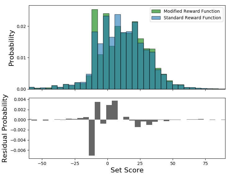Modifying the reward function has no significant effect on the distribution of set scores.

Interacting with the Network

We have now explored the high-level strategy choices of the network at length. Although there are always more metrics that one can use to quantify the strategy of the network, we have a good understanding of how it operates on a macro level. However, we are still missing a very important metric. How does the network perform against a human opponent? We have spent a lot of time learning about how the network approaches the game, but we still do not know if we should be learning from the network ourselves.

We need some way of convenient interacting with the network. Handcrafting individual game states and comparing our choices to those of the network, like we briefly explored in the previous article, is too time-intensive to be useful in providing a meaningful characterization of the performance of the network. The easiest solution is to make a simple command-line interface that is able to translate between the one-hot state representation and a representation that humans can understand. However, playing against the network through a command line is tedious. Especially since we will need a large number of games to form any conclusions given the stochastic nature of the game.

The next idea would be to make a simple GUI that I could use to play against the network. I prototyped a quick GUI using PyQt4, and a screenshot is shown below. In this layout, the discarded cards of each suit are shown on the left. The center of the screen shows the hands of both players as well as the deck, and the right of the screen shows the played cards of both players.

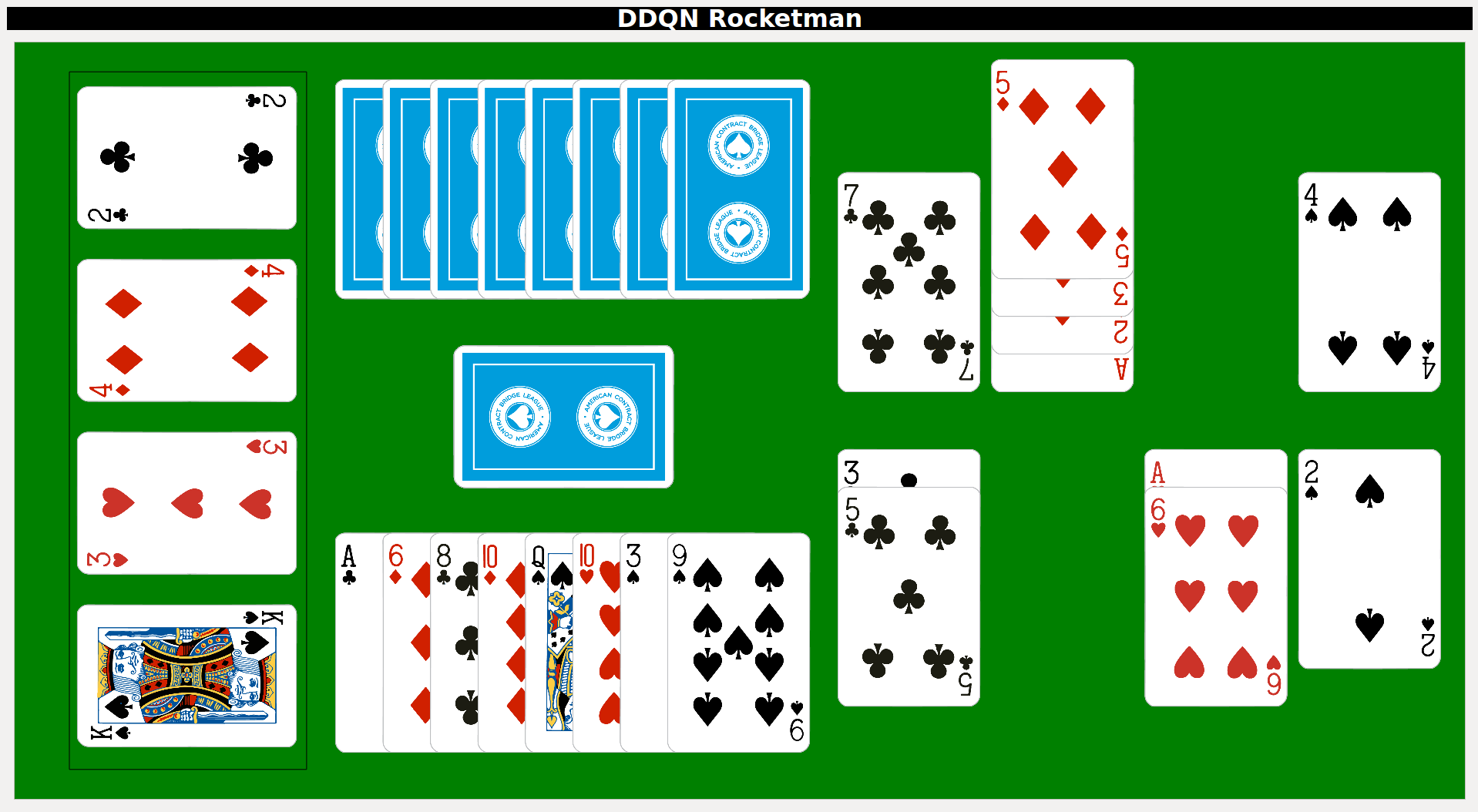Screenshot of the GUI created to interact with the trained network.

The GUI that I created was usable but buggy. Even ignoring the bugs, this approach did not feel right. I really wanted a network that I could physically play against using physical cards. Not only would this make playing against the network much more fun, it would also provide an excuse to have another machine learning project in computer vision. With this in mind, I decided to learn how to train a network to recognize standard playing cards.

Object Detection to Recognize Cards

Recognizing playing cards could quickly become a large standalone project, so I wanted to avoid reinventing the wheel as much as possible. While exploring different repositories, I found a repository for generating a dataset of playing cards that could be used with standard objection detection architectures. The repository contains a single comprehensive Jupyter notebook that converts videos of playing cards to individual card images and performs the necessary preprocessing of the images. The corners of the images are then used to generate the convex hull containing the rank and suit of each card. Finally, artificial training scenes are generated, and the bounding boxes are saved using the position of the convex hulls.

I will not explain process of generating the training data in more detail because the notebook is very well-written to explain the individual steps and also guide the interested user to perform all of the steps. Moreso, I cannot take any ownership for the code. Instead, I will briefly illustrate the different steps using the data that I recorded for use with this notebook.

Recording Card Videos

I first recorded roughly thirty second long videos of all of the individual cards in the deck. The purpose of the video was to capture the face of the card in different light conditions, so that the object detection network is not ultimately sensitive to light levels or illumination. Through experimentation, I found that I had best results if I recorded two individual videos, one at close range and another from further away. This was necessary for me because I was using a very cheap webcam that I purchased for this project. The camera did not focus properly, so the cards appear very blurry at close range. Gathering these additional scenes were crucial for the object detection to work with the webcam at different distances. An example of the video recorded at close range is shown below. Throughout the video, I try to vary the illumination to have a wide diversity of training images for a given card.

Extracting Card Faces

The card faces are then extracted from the individual video frames. Each video produces around 1000 individual card faces, a handful of which are shown in the image below. We can clearly see variety in the light levels and reflection in these images.

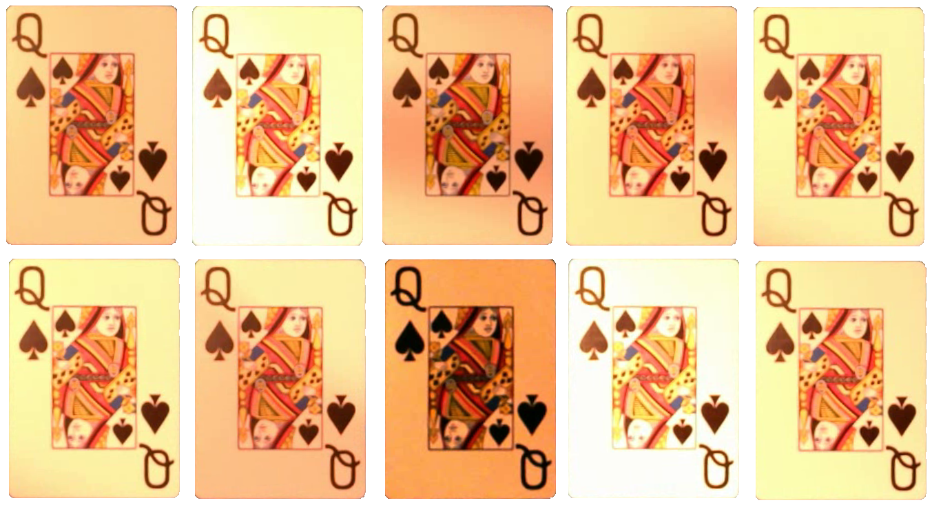Examples of the extracted card faces.

Generating Training Data

First, the convex hulls containing the rank and suit are identified on each card, as in the example below. These positions are saved, and then artifical scenes containing multiple cards against some random textured background are generated. Because the position of all of the convex hulls is known, the appropriate bounding boxes for each scene can be calculated. An example of an artificial scene with the calculated bounding boxes is shown below.

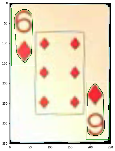Example of the convex hulls containing the rank and suit overlayed on the extracted card face.

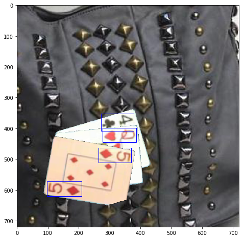Example of an artificial scene with bounding boxes that can be used to train an objection detection network.

Object Detection

At the end of this process, we have 100,000 artifical scenes containing a variable number of playing cards. Importantly, we also know the coordinates of the proper bounding boxes for each scene. We can then use this training set to train a network that predicts bounding boxes and then predicts the object classes from the bounding boxes. There exist several approaches to this, but I chose to use Yolo v3, which is both very fast and accurate. The speed is particularly appealing compared to alternatives, since we will be using the same computer to perform object detection and to evaluate the deep Q-network. In particular, I using the darknet implementation of Yolo v3, which implements several performance tweaks to the Yolo v3 architecture.

I trained the Yolo v3 implementation using 90% of the artifical scenes, and used the other 10% for validation. The network had very strong performance on the validation set before the training was finished (obtaining a mean average precision greater than 0.99), so I stopped it after 20,400 iterations. To demonstrate the trained network, I can input a previously unseen image such as the one below into the network. It is worth noting that all of the artificial scenes contained at most 3 cards, so this image is considerably different from the training data in this regard.

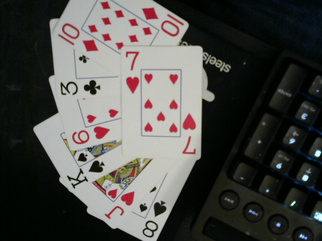Unseen image used to test the trained Yolo network.

After inputting this image into our trained network, we can get an annotated version with the predictions of the network overlayed. In the image below, we see that the network identifies tight bounding boxes around all of the visible corners, and all of the labels are correctly assigned. The network assigns all of these labels with a confidence of at least 98%, so it is very confident in the labels assigned. Another important metric is the inference time, since this will determine the feasibility of real-time detection. After the network was loaded into memory, the inference took only 36 milliseconds, which is plenty fast for keeping up with a card game played at a normal speed.

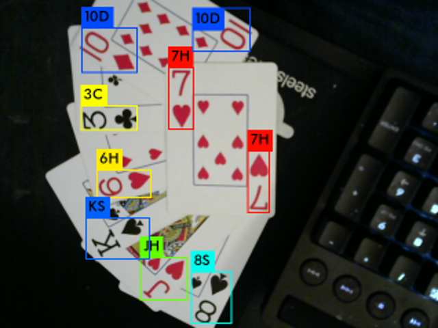All of the cards are properly labeled with tight bounding boxes.

We can demonstrate the speed of the inference by trying real-time detection. In the video below, we see that the labels are determined very quickly and are almost always correctly identified, even when the relevant information is partially obstructed. Also, the inference is able to process the images at around 15 frames per second, even when a large number of cards are present.

Finally, we can also look qualitatively at how robust the detection is. One can imagine that brightness, orientation, occlusion, movement, and distance could all affect the quality of the objection detection. In the video below, I try to introduce many of these problematic cases. We see that the network almost always correctly identifies the correct label. When the label is incorrect, the confidence is low and the correct label is quickly recovered. This bodes well for using our object detection system to accurately form game states from images of the cards.

Equipping our Agent with Vision

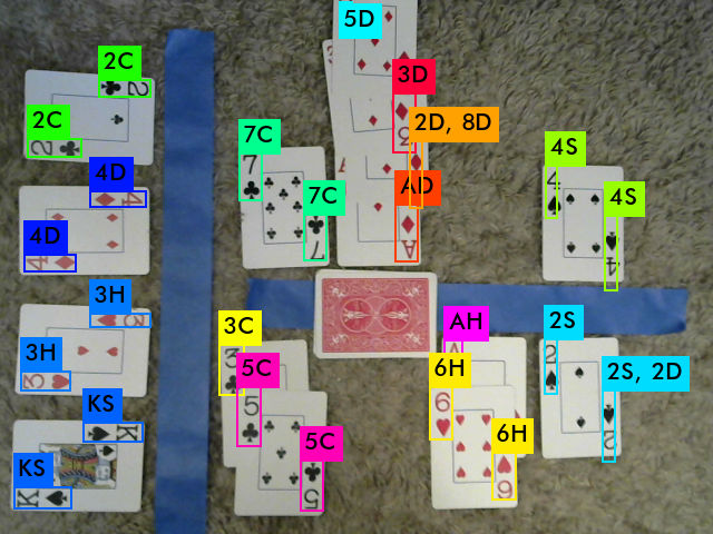
We now have an agent trained to play Lost Cities and also an object detection network trained to to recognize playing cards. All we have to do now is glue them together. To enable our trained agent to properly make decisions from the the visible cards, we need two webcams. One to view the hand of the agent, and another to view the public information of the game. Reading the hand is trivial now that we have our Yolo network properly trained. Processing the public information is slightly more challenging, though, because cards need to be properly assigned to one of three categories—discards, cards the agent has played, and cards the opponent has played. An example of the public game state information is shown below.

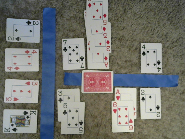Public information that must be processed for use with our trained agent.

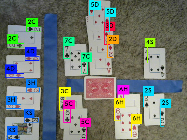
As the painter’s tape suggests, I went with the simplest solution for assigning the proper category to the visible cards. I used the recorded positions from the bounding boxes to determine the appropriate category for each card. There is a vertical divider used to determine if cards belong to the discard or played category and a separate horizontal divider used to determine the owner of the played cards. The painter’s tape is to help humans visualize the invisible boundaries, which are shown below, and is not used by the network.

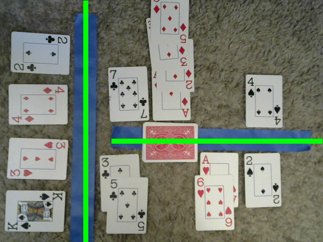Overlaying the boundaries used to categorize the public cards.

Finally, we use the trained Yolo network to identify all of the played and discarded cards. When this is combined with the positional information, we can correctly process all of the public information. When we combine this public information with the separate image containing the hand cards, we have everything needed to encode our observation of the game state in a form that can be evaluated by our trained agent.

The Yolo network correctly identifies all of the visible cards.

Challenging the Agent

In theory, we now have everything required to play a physical game of cards against the agent trained with a deep Q-network. The darknet implementation of Yolo v3 allows the user to create a shared library usable by Python from the C++ code. Because many frames are recorded before the game state changes, I stored the frames from both webcams in queues. Specifically, I used multiprocessing queues to help distribute the webcam capture, object detection, and trained agent evaluation across different threads. One thread captured frames from the webcams, another evaluated the Yolo network, and a third evaluated the agent with the information obtained from the object recognition.

I played a few games against the trained agent, and it won about as many as it lost. I want to play a large number of games against it to better quantify its performance, but playing against the agent is very difficult. The issue is that the card detection is not as robust in practice as it seems in our synthetic tests. As an example, the objection detection is shown for the frame taken moments before the above image below. We see now that the ace of diamonds is missed completely, even though the two images look identical to us.

The Yolo network frequently fails to detect a card…

And if we look just a few frames later, we now see that the ace of diamonds is missing again and now the 2 of diamonds and 3 of diamonds are not recognized either.

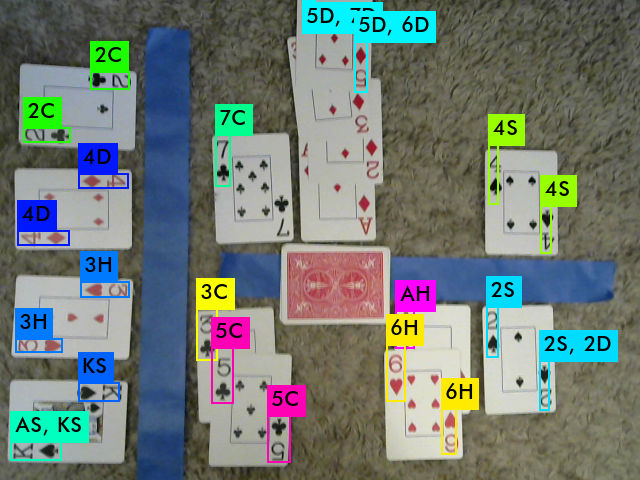…and occassionally misses multiple cards.

We have some hope in filtering out these bad examples, since we have access to the entire queues of frames. However, the errors were too frequent to be filtered out effectively. If we reduce the confidence threshold on the network, we eventually begin to detect this cards, but we introduce way more artifacts as well. So the network that we have trained is not quite robust enough to painlessly interact with our trained agent.

I believe that the network is not performing as well as it could be because of our training data. Through playing around with the object recognition, I found two specific shortcomings. First, the network struggles when the cards are too far away, as shown below. This is partially an issue because of low quality of distant targets in the frames captured by the webcam. This became an issue because our training data did not include enough artificial scenes where the cards were relatively small and/or blurred. These frames are unavoidable in practice, because there are so many cards that are visible to both players. We need to adjust the image augmentation to generate more of these training scenes.

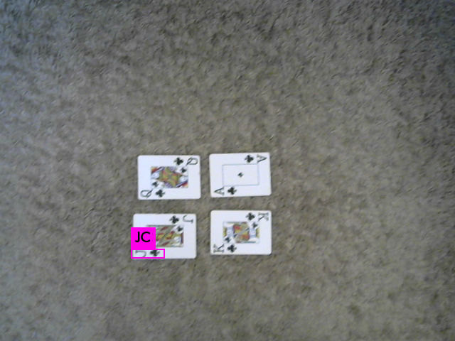The network performs poorly when cards are too far away.

The second issue pertains to the ordering of cards within a set. The augmentation used to generate the training scenes applied random rotation so that the network could recognize cards at any angle. However, most of the cards visible to both players are ordered in a column. Columns of cards make up most of the frames requiring detection, but they were not well-represented in the training set. For this reason, we also need to adjust the image augmentation to generate proportionally many more artificial scenes with stacked cards. We see a clear example of this being problematic in the previous section.

Conclusion

In the first half of this article, we learned how the agent was forming its strategy choices in Lost Cities. The agent generally opts for four short stacks, each of which results in a score drawn from a distribution with positive expected value. The strategy of the network is generally risk-averse, with relatively few sets resulting in large positive or negative scores. We also checked that these strategy choices were not a feature of the specific scoring function used but instead represents the attempt of the network to find an optimal solution despite the imperfect information nature of the game.

To gain a better sense of the performance of the agent, we trained a separate network to recognize playing cards in the second half of the article. From videos of card faces, we used image augmentation to generate a large number of artificial scenes. This dataset was then used to train a Yolo v3 network to perform object detection, finding the rank and suit information from the corners of cards. It generally performed well in synthetic tests, but in practice the object detection was not robust enough for use with our trained agent. In the future, I want to tune up the image augmentation so that we can achieve accurate recognition in practice. I can then more carefuly evaluate the performance of the deep Q-network trained on Lost Cities.

Accompanying Code

The code for this project is hosted on my Github account. The code sets up a gym environment for Lost Cities and learns to play the game using the deep Q-network described in this article.