Incan Gold: Deep Counterfactual Regret with Monte Carlo Tree Search
Introduction
Incan Gold is a very simple strategy game that requires players to balance risk and reward. Each player has two available actions at any time: protect the rewards obtained in the current round or risk them to obtain even more. Importantly, the rewards of future cards depend strongly on the actions of other players, since rewards are split among all of the active players. Although there is a large amount of randomness in the game, players rapidly discover a strong strategy due to the simplicity of the rules. But how strong is this strategy? Is there an optimal strategy for this game? I used a combination of Monte Carlo tree search and deep counterfactual regret minimization to try to answer these questions.
Game Description
First, I will briefly explain the structure of the game. The game supports a variable number of players, and the strategy choices slightly change with the number of players. A complete set of rule can be found here, but I will briefly explain the game in this section. The game is divided into five rounds, and at the start of each round all of the players start in the temple. Each round has multiple turns, which consist of turning over a new card that corresponds to exploring the temple. There are three different types of cards that can be revealed
- Gem card: Gems are eventually divided among all exploring players. Remaining gems are left to be divided among future leaving players.
- Artifact card: This card is worth 5 or 10 gems, depending on how many artifacts have been claimed, but can only be collected if a single player leaves the temple.
- Hazard card: When the second hazard card of the same type is drawn, all players still exploring leave the temple without any gems. Each turn continues until two of the same hazard card have been drawn or all players have left the temple. The player with the most gems at the end of the five rounds wins the game.
Learning from Game Theory
The optimal strategy for a given player to maximize his or her gem count depends strongly on the policy taken by other players—for instance, if one player is very risk-tolerant, there is considerable utility to be gained from leaving earlier to claim all of the artifacts and unclaimed gems. These observations suggest that there may be some interesting types of strategy supported by this game. However, they are only observations. Can we formalize our intuition and gain a more rigorous understanding of the game?
To properly study Incan Gold, we can turn to the field of game theory. The first major distiinction that we find from game theory pertains to the level of information available to players. Pefect information games, such as chess, provide players with all of the possible information needed to understand the current state of the game. Imperfect information games, on the other hand, have some element of the state that is unknown to the players. Incan Gold falls under this second category, since the players do not know the order of the cards in the deck and instead rely on the results of chance.
Because of this chance, players in general are not able to map their observed information to a unique state. Instead, players can only form a number of possible states consistent with their information. In the terminology of game theory, these indistinguishable set of states are termed “information sets.” For a given information set $I$, each player can from a policy $\sigma(I)$, a probability vector over the available actions. By enumerating over all of the possible infosets in the game, we can define $\sigma_p$, the complete policy for player $p$. To evaluate a policy, we can form a utility function $u$ quantifying the expected payoff. However, this expected payoff can only be calculated if the policy of other players is known. If we use $\sigma_{-p}$ as the policy of all players other than $p$, we can form the expected payoff for player $p$, $u_p(\sigma_p, \sigma_{-p})$, provided that player $p$ plays according to policy $\sigma_p$ and all other players play according to policy $\sigma_{-p}$. We now have the necessary framework for evaluating different policies from multiple players in an imperfect information game such as Incan Gold.
We can now use this foundation to build up quantities of interest to us. The first idea that we want to explore deals with how we can optimally play if we know the strategy of our opponents. This is called the “best response” to the opponents’ policy $\sigma_{-p}$ and is represented as $BR(\sigma_{-p})$. The best reponse is defined as
$$ \begin{align}u_p(BR(\sigma_{-p}), \sigma_{-p}) = \max_{\sigma_p’} u_p(\sigma_p’, \sigma_{-p}) \end{align}. $$
To illustrate these ideas, let’s look at the game of rock-paper-scissors. Although this example will be exceedingly simple, it should nicely illustrate the ideas that we will use to describe more complex games. If our opponent’s strategy profile $\sigma_{-p}$ is such that they deterministically play paper, our best response to that strategy is to play scissors. We can prove this mathematically if we define the payoff for the game. If wins are rewarded as +1, draws as +0, and losses as -1, we can optimize our policy, which we represent as the vector
$$ \sigma_p = \begin{pmatrix} P_{\text{rock}} \\ P_{\text{paper}} \\ P_{\text{scissors}} \end{pmatrix}. $$
Then our utility function is given by
$$ \displaylines{\begin{align} u_p(\sigma_p, \sigma_{-p}) &= u_p\Bigg(\begin{pmatrix} P_{\text{rock}} \\ P_{\text{paper}} \\ P_{\text{scissors}} \end{pmatrix}, \begin{pmatrix} 0 \\ 1 \\ 0 \end{pmatrix} \Bigg), \\ &= -1 \cdot P_{\text{rock}} + 0 \cdot P_{\text{paper}} + 1 \cdot P_{\text{scissors}}. \end{align}} $$
Because the strategy profile $\sigma_p = (0, 0, 1)^T$ trivially optimizes our utility function, it is the best response for the opponents strategy of always playing paper, matching what we intuitively know to be the answer.
Typically, however, we do not know the strategy profiles of the other players. So we require a more robust way to understand the relative merit of different strategy profiles. For this, we turn to the idea of a Nash equilibrium. This is the set of strategy profiles for which every player is playing the best response. Mathematically, the Nash equilibrium $\sigma^*$ is defined according to
$$ u_p(\sigma_p^*, \sigma_{-p}^*) = \max_{\sigma_{p}'} u_p(\sigma_p’, \sigma_{-p}') \hspace{1em} \forall p. $$
In words, this is the set of strategy profiles for which no player can profit by deviating. We can illustrate this concept too by rock-paper-scissors. The Nash equilibrium is given by $\sigma^* = (1/3, 1/3, 1/3)^T $, so that each player is playing all three options randomly with equal probability. In the interest, I will not cover a formal proof here. However, this is an intuitive solution if we think in terms of the exploitability of any strategy. If our opponent is more likely to player paper than rock, for instance, we can exploit this behavior and profitably deviate from our uniform probability distribution by playing scissors more often.
There are many interesting properties of Nash equilibria that are beyond the scope of this article. The key property of interest to our goals is that calculating a Nash equilibrium for Incan Gold means we have found a policy that we cannot outperform and does not allow our opponents to exploit our policy. This is “solving” the game in some sense, since we can only be penalized by playing any other strategy if our opponent(s) are also playing the optimal strategy. There are theoretical concerns, such as the possibility of multiple Nash equilibria, as well as practical concerns, since the Nash equilibria is only the optimal strategy if the opponent is also playing optimally. In practice, however, finding a Nash equilibrium provides us with a very strong strategy profile that allows us to win against our opponent(s) in expectation.
Solving for Nash Equilibrium
After establishing what a Nash equilibrium is and why we are interested in finding it, let’s figure out how to accomplish this. One may be tempted to just throw a reinforcement learning algorithm at the problem and hope to arrive near the optimal policy, since reinforcement learning has been successful in learning good strategies in many games. However, most reinforcement learning algorithms struggle to converge to good policies in imperfect information games. Instead, we will stick with the game theory approach and use an iterative algorithm called Counterfactual Regret Minimization that has been successful in solving many types of games.
I will not formally explain this algorithm, as many comprehensive papers already accomplish this. I advise the interested reader to study this paper for a formal introduction to Counterfactual Regret Minimization. Instead, I will attempt to intuitively explain how the algorithm works here. The first important idea is that of regret, which quantifies how much we regret playing a certain action. For instance, if we return to rock-paper-scissors and assume we played paper while our opponent played scissors, we regret not playing scissors, which would result in a draw instead of a loss. And we even more strongly regret not playing rock, which would have resulted in a win rather than a loss. Regret measures the difference between the utility resulting from a particular action and the utility of the action that was chosen.
We can use our measured regrets to inform future play. We would ideally like to play a strategy that minimizes our expected regret over many games. One way we can hope to accomplish this is to choose actions proportional to the the cumulative regrets, after some normalization. In the above example, we would be more likely to play rock on the next turn since this action is the one we most regretted playing. One can imagine using a procedure of this type to converge to an optimal policy in some games. This procedure is called “regret matching”, and it works well for simple games such as rock-paper-scissors.
Counterfactual Regret Minimization (CFR) builds on this idea for use in sequential games, in which a sequence of actions are required from each player for the game to end, and imperfect information games, in which the state is not uniquely known. To account for imperfect information, the algorithm also factors in the probability of reaching different information sets given the strategies of the players. And to account for the sequential aspect of games, the algorithm factors in information about both past and future states. The algorithm looks forward in time to estimate the probability of the different game states that can be reached given the probability of action sequences from each player. And when a terminal state is reached, the payoff is propogated backwards to previous states to inform future play.
Illustrating CFR Through Decision Trees
Because I am more interested in the readers understanding the CFR algorithm at a high level, I am not going to describe the algorithm more formally here. But I do wish to illustrate the ideas in the above paragraph to aid understanding. Before I can do this, however, I need to introduce the idea of a decision tree. For our purposes, a decision tree is a useful way to model any game that helps us to perform CFR. A decision tree consists of nodes, which represent opportunities for multiple outcomes to follow, and branches between causally-related nodes. Nodes can be decision nodes, in which a player must use his or her policy to choose among available actions, and chance nodes, in which a random event is chosen. There also exist terminal nodes, which represent the end of the game and assign the payoff to all players.
Continuing with the example of rock-paper-scissors, we can represent the decision tree we would face in the diagram below. Here we use green circles to represent decision nodes that allow us to choose an action, red circles to represent decision nodes of our opponent. Each decision node has three child nodes, one for each action choice. Each branch has a probability associated with playing the corresponding action. Following the action of player two, we arrive at a terminal node, represented as a white square. Each terminal node contains a tuple of the payoff given for both players. As we can see here, decision trees allow not just a convenient illustration of the different outcomes but also a compact description of the game of rock-paper-scissors.
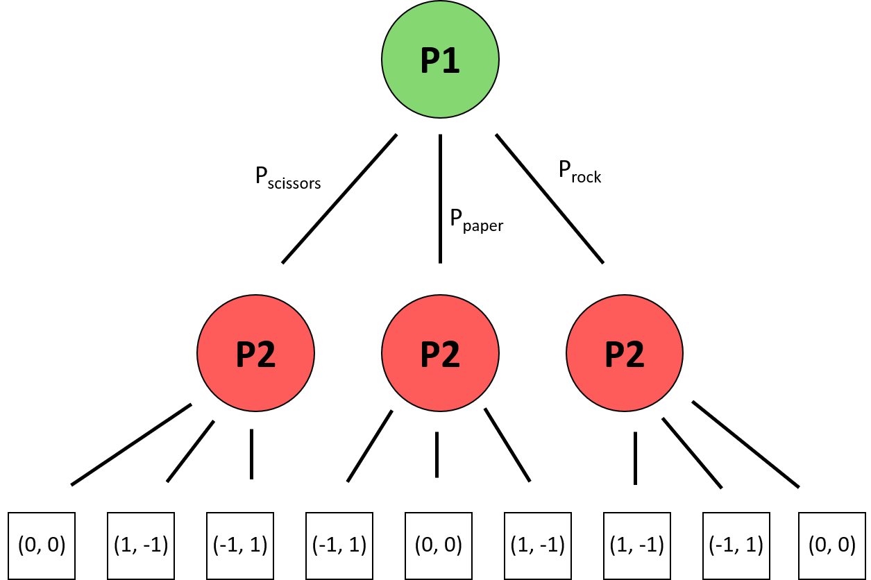 The decision tree representation of rock-paper-scissors.
The decision tree for Incan Gold is more complex due to the fact that the game also has imperfect information introduced through chance nodes and is sequential, so that many actions may be required from a player before a terminal state is reached. A condensed view of the decision tree after a single turn is shown below, with chance nodes shown as blue circles.
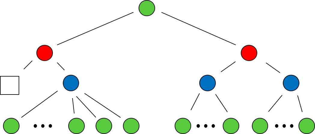 The decision tree representation of the first turn of Incan Gold.
To better understand the CFR algorithm, I will use a decision tree for an extremely simplified series of possible events in a single round of Incan Gold. To reduce the number of nodes in the tree, we will fix the actions of the opposing player to always continue to explore the temple. Furthermore, we will also fix the outcome of the chance nodes, since these introduce a high degree of branching. We will assume that a gem card of value 7 is drawn in the first round and that the next two cards drawn are both hazard cards of the same type, terminating the round. The decision tree for this specific situation is shown below, where we use the convention that the choice to explore leads to daughter nodes above the parent node and the choice to leave the temple leads to daughter nodes below. Note that after we have chosen to stop exploring, the decision tree still continues even though our action space has reduced to a single action for future turns.
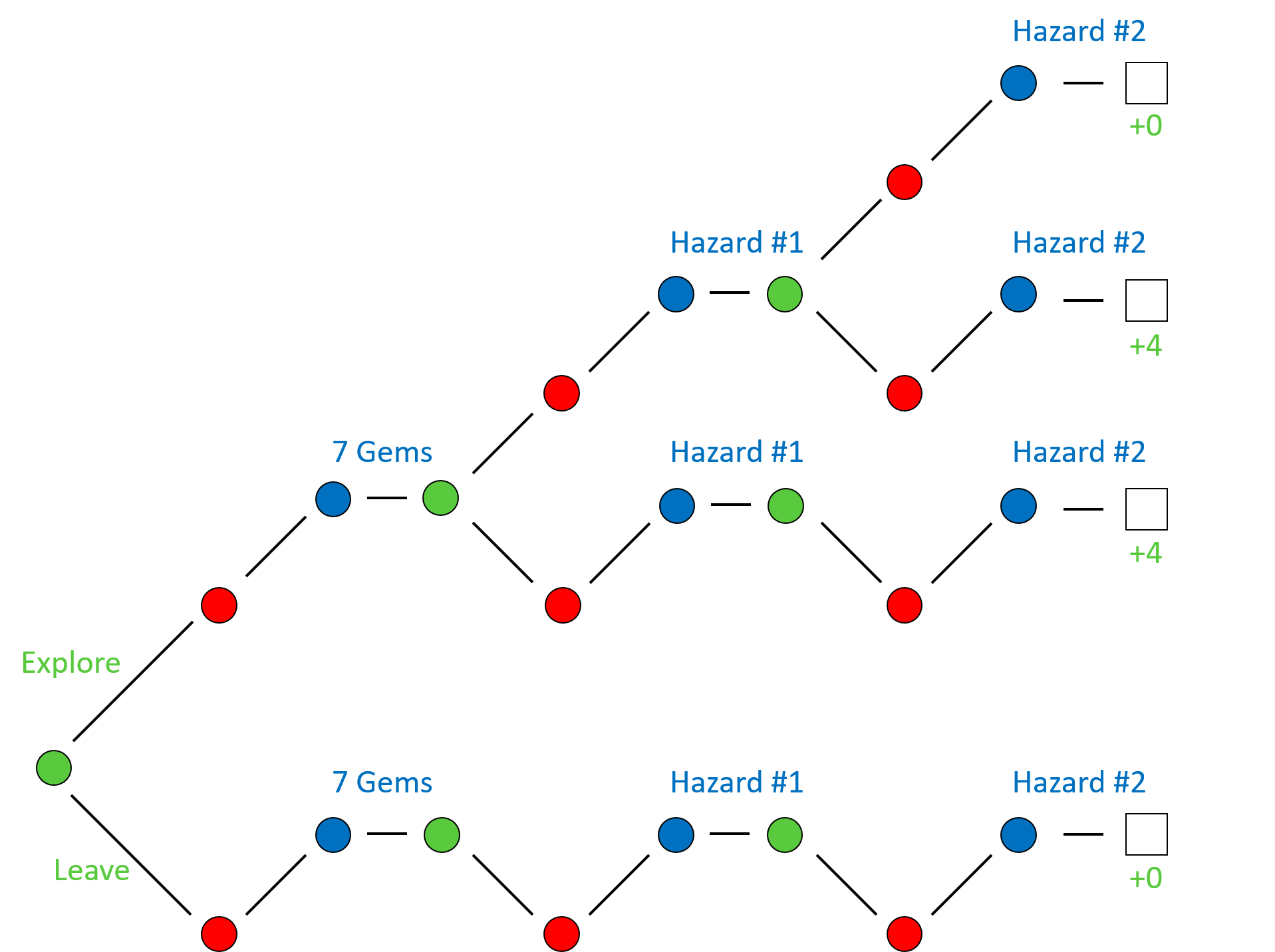 An example of a possible sequence of events if we freeze the actions of the opposing decision nodes and chance nodes.
We see that for this particular sequence of chance nodes, two of the branches lead to our player collected four gems. This is because the card with seven gems will be evenly divided between both players, leaving both players with three gems. If our player leaves the temple and the opposing player does not, our player will also get to collect the one remaining gem. However, our player receives zero gems if our player leaves before any gems are available or if our player remains in the temple after the second hazard card is played.
Now, let’s go through how CFR would work for this specific sequence. Let’s assume that we start with a policy that assigns equal weight to all of its choices. When we get to the end of the tree, we can calculate the regret associated with each sequence of choices, and propogate that information back up the tree to inform our policy for future decisions. For example, on the first decision node that we encounter, our player can explore the temple, which provides a mean utility of 8/3, or leave the temple, which provides a mean utility of 0. For this reason, our policy on the next iteration would preferentially weight the exploration choice at this node. The same logic happens at the second player node we encounter after exploring the temple—leaving the temple provides a mean utility of 4, while exploring the temple provides a mean utility of 2, so the policy is update to favor leaving the temple at this decision node. And finally, at the third decision node we encounter after choosing to explore on the previous turns, we see that leaving the temple carries a mean utility of 4 while continuing to explore carries a mean utility of 0, so that the next policy more heavily weighs leaving the temple at this decision node.
 An example of a possible sequence of events if we freeze the actions of the opposing decision nodes and chance nodes.
This hopefully illustrates the main idea behind CFR, but we have no reason to believe that this should converge to a stable policy. In the contrived scenario above, we quickly converge to an optimal policy simply by memorizing the tree. However, in a more realistic scenario, each chance node spawns a large number of daughter nodes, and each tree typically requires many more decision nodes. Both the randomness associated with the chance nodes and size of the tree should at least give us pause when expecting this algorithm to work. Luckily, proofs exist that this approach converges to a Nash equilibrium in two-player zero-sum games, and it has been used successfully in many games that do not satisfy these assumptions. For instance, a variant of this idea has been used in the algorithms that exhibited super-human performance in both the games of poker and go.
Deep CFR
Coming soon, along with results.