Lost Cities: Using Deep Q-Networks to Learn a Simple Card Game
Introduction
While presenting my research at conferences, I often ran into a friend from Caltech who was also working in biophysics for his PhD. After the talks had finished for the day, we were looking for some sort of two-player game we could play together. Through a process of trial and error, we eliminated all but a simple card game inspired by the rules of the board game Lost Cities.
The rules of the game are quite simple, and we seemed to have quickly discovered a strong strategy. Or at least I did…the first night we played, I won the majority of the matches and questioned the strategic reasoning of my friend. However, the next night we played, I lost the vast majority of the matches, much to the enjoyment of my friend, despite no major shifts in either of our strategies. This got me interested in wanting to know more about the game. Were the rules so simple that the winner was largely stochastic with reasonable play? Or was there a single strategy that would win in expectation value against all others? Or did the game support multiple distinct strategy policies that formed some sort of Nash equilibrium?
While these questions lead to lots of discussion, we had no way of answering them definitively. The game was too obscure to have expert players who had played thousands of matches, and the state space was prohibitively large for any sort of meaningful analytic progress. But maybe a computer could play thousands of matches? At this time, I knew little about neural networks or many other details of the field of machine learning, but I had the perfect problem to motivate me to learn more.
Game Rules
The rules of the card game are quite simple. Each player has five cards in his or her hand, and players score points based on the cards played from their hand. Players are allowed to form any number of stacks of cards, each of which can only contain a single suit. Additionally, cards must be added to each stack in increasing value. Finally, face cards and aces can be played before any number cards, which serve to multiply the score of a given stack. Each stack is scored according to
$$ (N_{\mathrm{multipliers}} + 1) * (\Sigma - 20) $$
where $N_{\mathrm{multipliers}}$ is the number of face cards played before any numerals and $\Sigma$ is the sum of the numerical cards in that stack. An illustration of how a stack is scored is shown in the image below. The penalty of twenty points per stack requires players to carefully consider starting a new stack. Summing the different scores from all stacks results in the game score for each player. There are two additional wrinkles to this, though. First, there is an additional additive reward of twenty points (not subject to the effect of multipliers) for any stack with eight or more cards. And secondly, the player has the choice of counting the ace as a “1”, if and only if is immediately preceding the first numeral card.
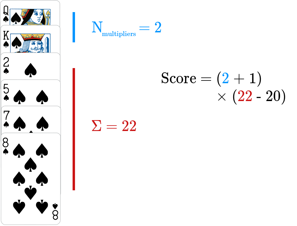 Illustration of how a stack is scored.
The deck of cards consists of a standard 52-card deck. Players alternate turns until there are no cards left in the deck. On each turn, each player must either play a card from his or her hand or discard a card from his or hand. The player then draws either a new unknown card from the top of the deck or one of the face-up discarded cards. There is a separate discard pile for each suit.
Essentially, each player is trying to perform a complex optimization problem trying to balance risk and reward. Large scores can only be achieved by large stacks of numerals on top of multipliers. However, large negative scores can also be achieved by playing multipliers without enough numeral cards on top of them. The problem is made complex by the severity of the imperfect knowledge—at the start of the game, players only have knowledge of the five cards in their hands. For this reason, players must try to estimate the number and value of numeral cards that they could draw before investing in creating a new stack.
Finding Policies with Reinforcement Learning
At a high level, this card game can be described as two agents making actions to try to maximize their rewards. The actions are informed by their observations of the state of the game. With this choice of language, this problem seems like a very natural fit for reinforcement learning, an area of machine learning concerned with understanding how agents maximize their cumulative rewards as they interact with some environment. We can hope to use reinforcement learning to find a policy for each agent that maps its observation to the action that will maximize its expected rewards.
In formulating this problematic mathematically, it is convenient to define a function $Q(s, a)$ that estimates the total reward we would expect to achieve by performing action $a$ from initial state $s$ and then following some determined policy. For our problem, the state space is combinatorically large, so we cannot expect to store an individual value $Q(s, a)$ for every possible state and action. Instead, we seek to approximate this function using a neural network. Because of the universal approximation theorem, we can hope to reasonably approximate our $Q$ function with a neural network.
If we imagine that we can approximate any evaluation of our $Q$ function, how would we use this to inform our policy? Intuitively, we would want to simply choose whichever action maximizes $Q(s, a)$ for our particular state $s$. We can capture this same idea if we imagine that each action results in some immediate fixed reward $r_0$ as well as a number of future rewards $\{r_i\}$. For generality, we will assume that future rewards might be weighted differently according to their horizon. To accomplish this, we discount future rewards by a factor $\gamma$ so that we can write our optimal policy as
$$ Q^{\ast}(s, a) = r_0 + \gamma r_1 + \gamma^2 r_2 + \cdots $$
By using the definition of the optical policy, we see that we can equivalently write this expression recursively as
$$ Q^{\ast}(s, a) = r_0 + \gamma \max_{a'} Q^{\ast}(s', a') $$
if we let $s'$ represent the state we are in after taking action $a$ and $r_0$ the subsequent reward. This is a motivation (not quite a true derivation) of the Bellman equation.
The Bellman equation is very useful for us because it informs us how we should be updating our estimation of $Q(s, a)$. If we start with some randomly initialized $Q(s, a)$ and take a step in our system, we will perform some action $a$ from initial state $s$ to final state $s'$ that produces some reward $r$. Using this values, we can update our estimate of $Q$ according to
$$Q^{\mathrm{final}}(s, a) = Q^{\mathrm{initial}}(s, a) + \alpha \cdot \gamma Q(s', a)$$
for some step size $\alpha$. We hope that by performing many steps in our environment, we can eventually converge to $Q^{\ast}$, the expected future rewards with an optimal policy.
The process we have described above is called a Deep Q-Network (DQN), where we train a neural network using reinforcement learning through self-play to be able to estimate $Q(s, a)$ for any pair of states and actions. The power of DQNs was first illustrated in a groundbreaking paper by Mnih et al. in 2013. In this paper, the authors achieved high levels of performance in several Atari games using this idea. The results of this simple algorithm give us hope that we can deploy a similar solution to playing Lost Cities.
We have the added benefit of utilizing additional years of progress on DQNs. The two main ideas we incorporate are experience replay and double DQNs. Experience replay provides our algorithm with an efficient way of using the stored samples. Rather than sample them uniformly, prioritized replay assigns priority to those that deviate most from the current estimate of the Q function. Double Q-learning introduces a second network that is also trained to estimate the Q function. By using a second network, we can estimate the Q function with less bias and in a way that leads to more stable convergence. For a more comprehensive intuitive explanation of these improvements, I direct the curious reader to an excellent summary by Jaromír Janisch, whose article inspired much of the high-level design of my own implementation.
Game Representation
My description of the rules of the game (hopefully) make sense to humans with a basic understanding of card games but requires translation into a form usable with a DQN architecture. We need to think carefully about the different representations we want for the game information. First is the game state, which completely specifies all of the cards in the game. Separate from the complete game state are the two observations of the players. There is considerable information not available to the players—cards in the hand of the opposing player, the cards remaining in the deck, and the order of these cards.
In our description of DQN, we loosely used $s$ to represent the state of the system. A more careful treatment would use the player observations. In some problems, the states and observations are equivalent. But for ours, the observation contains considerable less information. None of the math changes by using observations, so I did not add this additional complication. But in practice, the agents can only act upon the information available to them. If the agents knew the full game state, we would have no need for a DQN afterall.
In forming our observations, we need to balance being as descriptive as possible (within the information available to each agent) with having a reasonable number of unique identifiers. I came up with 11 unique identifiers for each card, which can be seen in the table below.
| Identifier | Card Description |
|---|---|
| 0 | Player 1 Hand |
| 1 | Player 1 Board |
| 2 | Player 1 Board Flex Play |
| 3 | Player 2 Hand |
| 4 | Player 2 Board |
| 5 | Player 2 Board Flex Play |
| 6 | Player 1 Discard |
| 7 | Player 1 Top Discard |
| 8 | Player 2 Discard |
| 9 | Player 2 Top Discard |
| 10 | Deck |
Just to reiterate, this set of descriptions is not sufficient for the true state of the game, since we have no knowledge of the order of cards. In fact, it is not even a complete description of all of the possible information available to the agents. If a card is in the discard pile, we only record if it is the top card or not. In reality, the order of these cards is public information. However, including such information should add little to the strategy of the agents and greatly increase the number of identifiers needed. We want to use as lean a set of descriptors as possible to minimize adding extraneous information into our neural network.
As an example of using this encoding, a typical state of the game may be represented as
$$ \left[ \begin{array}{c|ccccccccccccc} & A & 2 & 3 & 4 & 5 & 6 & 7 & 8 & 9 & 10 & J & Q & K \\ \hline C & 0 & 1 & 4 & 10 & 1 & 10 & 1 & 3 & 1 & 10 & 1 & 1 & 1 \\ D & 10 & 1 & 1 & 0 & 10 & 3 & 10 & 10 & 3 & 10 & 10 & 1 & 3 \\ H & 3 & 1 & 0 & 1 & 1 & 4 & 3 & 4 & 4 & 4 & 10 & 0 & 4 \\ S & 5 & 0 & 4 & 0 & 3 & 4 & 3 & 4 & 10 & 0 & 9 & 4 & 0 \\ \end{array} \right] $$
This state is not equivalent to the player observations, since players have no knowledge of the cards in the hand of the opposing player. The observations can be easily formed by mapping cards in the hands of opposing players to the same identifier used to represent unknown cards in the deck. We also use one-hot encoding to represent the observations, so the input observation size is a single vector with 520 binary elements.
We also need to form an encoding for the actions that players may take. On each turn, a player may either play or discard a card in their hand and also draw from either the deck or a discard pile. We have considerable flexibility with how we choose to encode this information. I settled upon using a three-tuple of the form
$$ (i_{\mathrm{card}}, j_{\mathrm{play}}, k_{\mathrm{draw}}) $$
where $i_{\mathrm{card}} \in [0, 51]$ denotes the index of the card to be acted upon, $j_{\mathrm{play}} \in [0, 1]$ denotes whether the card is to be played or discarded, and $k_{\mathrm{draw}} \in [0, 4]$ denotes the index of the location from which the card is drawn (deck or one of suit-specific discard piles). Note that there are restrictions on which values are allowed in this representation, since only certain indices are valid for a given game state. Using this action encoding, we can form a one-hot vector with 520 elements for the action choice.
Reward Function
To use reinforcement learning, we need to be able to represent actions, observations, and rewards. In the previous section, we formulated an encoding for both actions and observations that is usable by a neural network. The only remaining quantity that we need to define is our reward function. Initially, this seems trivial—we understand how scores are calculated, and scores are the quantity we most aptly want to maximize.
However, there are reasons to think that this is not the best reward function even though it is the most natural. The reason is that the scoring function is not monotonic with the cards played. Allow me to explain with an example. Imagine that we had a very promising hand in a particular suit, so we first play a multiplier to increase the scoring potential for the stack that we will build. If we simply evaluate the scoring function after this move, we went from 0 points to -40. We can see how this would present a challenge to our reinfocement learning algorithm. If we want to maximize the rewards, we would be better off discarding a card and staying at 0 points. And if we were to play another card on top of the multiplier in the following turn, we would receive another large, negative reward.
This challenge is certainly not insurmountable. One potential solution would be to only give the agent a reward when the game was finished. This eliminates the issue I described above and should truly allow the agent to optimize its final score, which is the only physical quantity of interest. However, this introduces another problem. Our reward function is now very sparse. For all but the final action, the agent receives no reward. And then when the game terminates, it has a single reward that it needs to figure out how to effective propogate to all of the intermediate states. In the limit of infinite training time, this is not an issue at all. But in practice, a sparse reward will make converging to a stable policy very difficult.
Finally, another solution would be to create an artificial reward function inspired by the scoring function. If we can craft an intelligent reward function, we can overcome both the reward sparsity and the bias towards risk aversion. However, the downside to this approach is that the quantity that we would be maximizing is not the true quantity of interest. We need to ensure that a large, positive value of the reward function is indicative of a large, positive score.
We will leave the specific choice of an artifical reward function as an open problem for now and experiment with different choices in our reinforcement learning training. We will just briefly touch upon two ideas that may be beneficial to produce the desired properties. First, we may want to include some quantification of scoring potential so that playing multipliers (when appropriate) has less of a valley to overcome. And second, we may want to perform some sort of temporal weighting so that the final reward function has a larger importance than the reward function early in the game. An illustration of what this could look like qualitatively is shown in the figure below, which compares the different reward functions for the stack illustrated above.
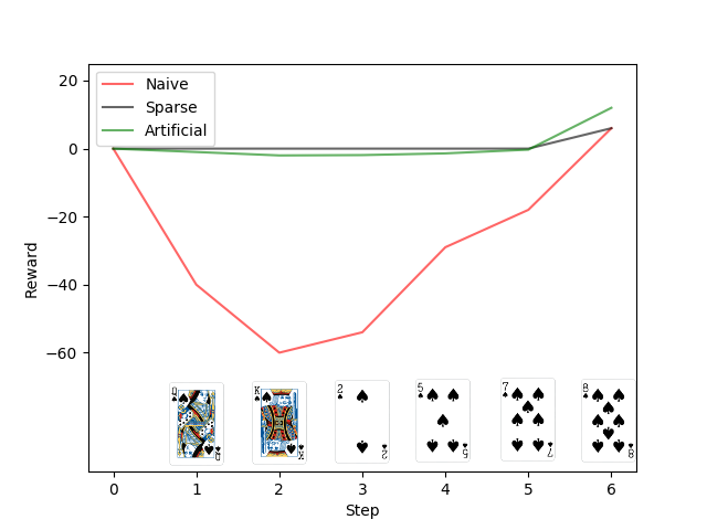 Comparing different candidate reward functions for use in training our agents.
Code
I created a Python implementation of Lost Cities that uses the popular Gym library as a base class, allowing standard off-the-shelf reinforcement learning algorithms to work with my custom environment. I next implemented a DDQN with prioritized replay in Tensorflow. The organization borrowed heavily from the previously mentioned set of articles by Jaromír Janisch. Since my implementation borrows so heavily from one that is already well-written, so I will not detail the specifics here.
I will, however, briefly mention some of the thought that went into the choice of hyperparameters. One important hyperparameter is the buffer size. Before the reinforcement learning agent begins to act, the buffer is initially populated with the results generated from an agent that chooses randomly among the valid actions at each turn. Since this random agent makes choices as quickly as a random number generator, it is tempting to use a very large buffer. Although we will never have a buffer large enough to represent every possible state, the prioritized replay still benefits from a large number of states so that it can choose many that are instructive for each new decision at hand.
However, we need to think about how many episodes we can reasonably expect to train our agent. Since I do not have access to a GPU, we are somewhat limited in terms of our computational power. If we hope to train our agents for $10^4$ episodes, each of which has $\mathcal{O}(20)$ decision points for each agent, we only expect to encounter $\mathcal{O}(10^5)$ new observations. If our buffer is too large, each decision point will be heavily biased towards actions chosen by the random agent. For this reason, we probably want a buffer that stores $\mathcal{O}(10^4)$ states.
Thinking about the number of expected episodes also helps us determine a reasonable value for the hyperparameter governing the balance between exploration and exploitation. We use an epsilon-greedy policy, in which the optimal action is chosen according to the Q-network with probability $1 - \epsilon$ and a random action is chosen with probability $\epsilon$. The value for $\epsilon$ is not hard-coded, but instead is annealed as the algorithm is run. This allows random actions to be taken almost exclusively initially when we have little trust the predictions from the Q-network but allow random actions to become rare once the Q-network has been sufficiently trained. The value for $\epsilon$ is annealed exponentially, with the rate chosen such that we have $\epsilon \simeq \epsilon_{\mathrm{min}}$ at the end of the expected $\mathcal{O}(10^4)$ episodes. The annealing schedule is shown in the figure below.
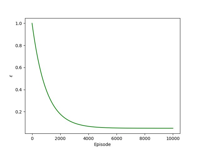 The “greed”
 $\epsilon$ is annealed to favor exploration early in the training and exploitation late in the training.
Preliminary Results
I first trained a simple network with two hidden layers each containing 512 nodes for our DDQN. This is likely not the optimal architecture for learning a policy for Lost Cities, but it provides a place to begin. The figure below shows the cumulative score of both agents using the DDQN as a function of the number of training episodes (complete games). We see that each player is averaging a score around 40 points, which is a very respectable score. There exists a lot of variance in the scores simply because the DDQN only has the respective player’s observation as its input. In the language of game theory, Lost Cities is an imperfect information game. The lack of complete information makes the game interesting, and it similarly results in very large variance in the scores obtained by human players.
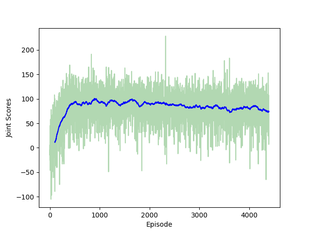 The mean joint scores collected by the two agents rapidly converge to a value near 83.
It is perhaps surprising that the network achieves such good scores from so few episodes. Clearly, the network is learning the structure of the game and is able to navigate the imperfect information to make intelligent choices. However, all of these results were achieved using the sparse game scores as the reward function, so that the majority of decisions do not receive any immediate reward. The network is able to propogate the Q-values back to intermediate states much quicker than I was expecting.
This is exciting, since we avoid the potential pitfalls that I discussed above in regards to sparse rewards. However, it is also almost disappointing, since we do not have much potential to improve our results through crafting a reward function. Just for my own edification, I wanted to try an alternative reward function to demonstrate the possiblities. I tried a reward function that instead relies on the maximum possible score that can be achieved from the given state. For each decision point, a discrete optimization is performed to determine the maximum score that could be achieved. To govern the reasonability of each sequence, cards are assigned a weight based on their location. Cards that are in the hand of the agent are given a weight of 1, cards that can possibly be drawn into the hand of the agent are given some weight $w < 1$, and cards that are already played are given a weight of 0.
I trained a new network using this reward function with $w = 0.4$, and the cumulative scores are shown in the figure below. We see that the mean scores are less than what we obtain when we use the scores as the reward function. This is to be expected, since we are not optimizing the scores in this case. Although the agent is trying to maximize its total possible score, this does not translate to larger maximum collected scores. We see this by comparing the score distributions obtained from the two different reward functions.
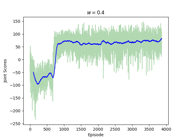 The mean joint scores collected by the two agents rapidly converge to a value near 68.
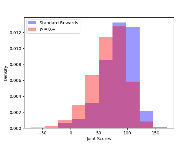 The distribution of final scores show that the natural reward function always leads to larger scores.
Although the alternative reward function is too crude to capture any useful ideas, one can imagine a situation in which a refined version of this reward function would be the better choice. If two players are playing an unknown number of games until one reaches some specified score, it may make sense for one player to play with a higher variance strategy if he or she would otherwise lose in expectation. So while this crude reward function that we crafted is likely not optimal for any goal, it does illustrate the potential utility of using an alternative reward function for specific situations.
Score Optimization
I spent considerable time trying to optimize the network architecture and various optimizer hyperparameters. After finding a good set of hyperparameters, I froze the values and instead explored the scores obtained with different network architectures using these common hyperparameters. This is far from a true hyperparameter optimization, which would require too much training time for my desktop computer without a GPU. However, we still observe interesting results in the table below. In general, it seems from these very limited results that network depth is important for achieving high scores. This is not surprising, since network depth adds additional non-linearity. We see that the number of tunable parameters alone is not particularly predictive of network performance.
| Hidden Layer(s) Architecture | Mean Joint Scores | Trainable Parameters ($10^6$) |
|---|---|---|
| 8 x 64 | 93.1 | 0.23 |
| 5 x 512 | 90.8 | 1.60 |
| 1 x 1024 + 3 x 512 | 83.0 | 1.73 |
| 2 x 512 | 82.9 | 0.81 |
| 2 x 1024 + 1 x 512 | 76.0 | 2.25 |
| 1 x 1024 + 1 x 512 | 72.8 | 1.20 |
| 1 x 1024 | 71.5 | 0.94 |
| 1 x 2048 | 54.6 | 1.74 |
| 8 x 16 | -0.6 | 0.16 |
With the 8 x 16 architecture, we seem to be reaching the limit of depth versus model size tradeoff, since the performance drops off steeply to approach that of a random agent. However, even this model does learn something, even if it is not obvious looking at the mean joint scores. In the joint scores plot below, we see that there is some structure as it tries to learn. Something strange happens around episode 920, which completely impedes its ability to gain positive rewards. This plot suggests that the model is not completely incapable of learning, but we would need to tune the other hyperparameters to allow it to properly learn.
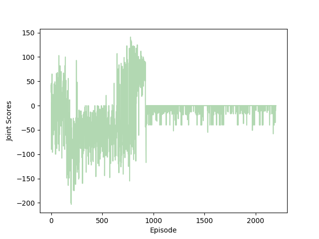 The joint scores collected by the 8x16 architecture are not without structure, suggesting that learning could be possible with a different choice of hyperparmeters.
Shortcomings
There is reason to believe that all of these results suffer from overfitting. The state space in the game is simply too large for a network to encounter every state. For example, the game state is the least complex at the start of the game, when there are no discarded or played cards. Even for this initial state, there are more than 750 million unique hands that a player could be dealt. A more advanced encoding would take advantage of the symmetry that exists among the four suits, and would also likely rely on bucketing to group together sufficiently similar states. With the huge number of states combined with the incomplete information, it is perhaps surprising that our crude approach works at all. We are expecting a huge deal of generalization from our network. Despite these issues, it is performing very well on hands it almost certainly has not seen before.
Overcoming this overfitting is not trivial, since most of the observed states are completely new to the network. One solution that I tried is adding dropout between the layers of 5x512 network. Generally, dropout is effective at reducing overfitting since the output of the network cannot be predicated on all of the possible features. However, in my limited tests, the network without dropout simply does not perform well. While dropout allows our results to be less heavily influenced by hands that it has observed, the resulting heuristics are even more imprecise. Generally, they were imprecise to the point of the network losing all of its ability to collect rewards. An example of the collected rewards from a 5x512 network with dropout is shown below.
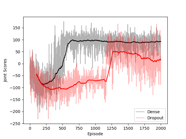 Adding dropout between the dense layers does not improve our scores despite reducing overfitting.
One direct consequence of this overfitting is that our Q-network is very susceptible to adversarial attacks. The fraction of encountered states is miniscule, so it relies on rough heuristics to evaluate a hand. The imprecision introduced by these heuristics means that for certain choices of states, the network does not perform in an optimal way. A very basic way to evaluate our network is to examine the predicted Q-values for all of the possible actions for a given state. For simplicity, we will look at the start of the game, where the initial state consists only of the hand of the player. It does not take many attempts to find a hand where the action taken by the network seems highly suboptimal. One troublesome hand for the 5x512 network, for example, is shown below.
 A troublesome starting hand for our Q-network.
We can encode this hand information into our state observation and predict the actions that maximize the Q-function as outputted from our network. There are sixteen valid actions—each of the eight cards can be either played or discarded. The Q-values from playing every card are higher than discarding that card. This is probably not quite correct, since playing the 9 of diamonds can never lead to positive points, but the general idea that cards should be played rather than discarded early in the game seems correct.
However, the results get more troublesome when we look at which cards the network prefers to play for this specific hand. Before we look at the predictions made by the network, let’s take a second to think about what we would do with this starting hand. The first choice would probably be to play the queen of hearts. We already have enough hearts in our hand to be guaranteed a positive score if all are played, so leading with a multiplier seems very safe. Perhaps even leading with the three of hearts is not bad, for much of the same logic. And finally, one could imagine playing the 2 of clubs. While not the strongest opening, we have a decent floor with the 8 of clubs also in our hand, and there are many other available cards that we could draw to add to the set.
Now let’s see how the neural network ranks the different playing options. In the figure below, I plot the Q-values of the network in order of its preferred cards to play. We see that the top three choices all fall outside of our expected moves. Additionally, we see that all of the Q-values are quite close to each other, so our network is not particuarly discriminating. This is perhaps good, since the network only expresses a slight preference for these suboptimal plays.
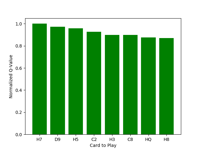 The Q-values for playing each card, as estimated by our well-trained network.
This single adversarial attack is interesting, but it raises more questions than it answers. First, how common are these adversarial examples? It seems like they cannot be exceedingly common, since the network is able to achieve good mean scores. But maybe the network is generally poor at the initial hands and has very strong play for the late game to end up with good scores. Exploring these different cases is difficult when we can only learn about the network response by forming initial states “by hand” and examining the network output. Learning about how the network responds to a given state is arguably the most interesting part of the project and also one of the most challenging. I intend to explore this more thoroughly in a follow-up article to better explore the network heuristics.
Conclusion
An agent using the best network architecture is able to achieve a mean score of 45 points, which is a very respectable score. To put this in context, an agent using a random policy obtains a mean score of -3 over 10,000 games. The ability of the network to learn a reasonable policy in so few games is perhaps surprising, given that there are so many unvisited states. Additionally, our methodology has been somewhat crude, so the performance of the Q-network is surprisingly decent given the imperfect information available to it.
Now that we have a well-trained agent, what can we do with it? I would like to see how it performs with given scenarios and try to learn some heuristics behind its strategy choices. And ideally, I would want to be able to play against it. This would serve as a true test of its performance, and it would allow us much greater insight into its decision-making. These are all ideas that I hope to explore in a future article, so look our for Part 2 if you are interested.
Accompanying Code
The code for this project is hosted on my Github account. The code sets up a gym environment for Lost Cities and learns to play the game using the deep Q-network described in this article.